Introduction
Many fundamental evolutionary processes, such as adaptation, speciation, and extinction, operate in a spatial context. When the historical aspect of this spatial context cannot be observed directly, as is often the case, biogeographic inference may be applied to estimate ancestral species ranges. This works by leveraging phylogenetic, molecular, and geographical information to model species distributions as the outcome of biogeographic processes. How to best model these processes requires special consideration, such as how ranges are inherited following speciation events, how geological events might influence dispersal rates, and what factors affect rates of dispersal and extirpation. A major technical challenge of modeling range evolution is how to translate these natural processes into stochastic processes that remain tractable for inference. This tutorial provides a brief background in some of these models, then describes how to perform Bayesian inference of historical biogeography using a Dispersal-Extinction-Cladogenesis (DEC) model in RevBayes.
Overview of the Dispersal-Extinction-Cladogenesis Model
The Dispersal-Extinction-Cladogenesis (DEC) process models range evolution as a discrete-valued process (Ree et al. 2005; Ree and Smith 2008). There are three key components to understanding the DEC model: range characters, anagenetic range evolution, and cladogenetic range evolution ().
Discrete Range Characters
DEC interprets taxon ranges as presence-absence data, that is, where a species is observed or not observed across multiple discrete areas. For example, say there are three areas, A, B, and C. If a species is present in areas A and C, then its range equals AC, which can also be encoded into the length-3 bit vector, 101. Bit vectors may also be transformed into an integer-valued state, e.g., the binary number 101 equals the integer 5. Note, add 1 to the value of the integer-valued state to access that state from a RevBayes object, such as a rate matrix, e.g. the range AC with integer value 5 is accessed at index 6.
| Range | Bits | Size | Integer |
|---|---|---|---|
| $\emptyset$ | 000 | 0 | 0 |
| A | 100 | 1 | 1 |
| B | 010 | 1 | 2 |
| C | 001 | 1 | 3 |
| AB | 110 | 2 | 4 |
| AC | 101 | 2 | 5 |
| BC | 011 | 2 | 6 |
| ABC | 111 | 3 | 7 |
The decimal representation of range states is rarely used in discussion, but it is useful to keep in mind when considering the total number of possible ranges for a species and when processing output.
Anagenetic Range Evolution
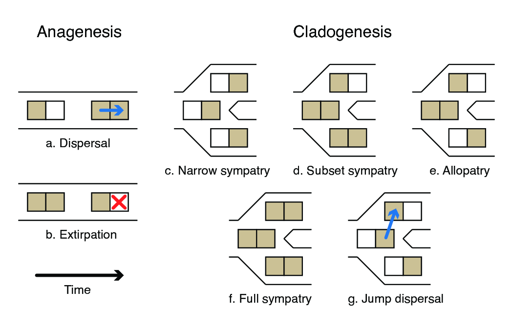
In the context of the DEC model, anagenesis refers to range evolution that occurs between speciation events within lineages. There are two types of anagenetic events, dispersal (a) and (local) extinction or exitrpation (b). Because DEC uses discrete-valued ranges, anagenesis is modeled using a continuous-time Markov chain. This, in turn, allows us to compute transition probability of a character changing from $i$ to $j$ in time $t$ through matrix exponentiation \(\mathbf{P}_{ij}(t) = \left[ \exp \left\lbrace \mathbf{Q}t \right\rbrace \right]_{ij},\) where $\textbf{Q}$ is the instantaneous rate matrix defining the rates of change between all pairs of characters, and $\textbf{P}$ is the transition probability rate matrix. The indices $i$ and $j$ represent different ranges, each of which is encoded as the set of areas occupied by the species. The probability has integrated over all possible scenarios of character transitions that could occur during $t$ so long as the chain begins in range $i$ and ends in range $j$. We can then encode ${\bf Q}$ to reflect the allowable classes of range evolution events with biologically meaningful parameters. For three areas, the rates in the anagenetic rate matrix are
\[\textbf{Q} = \begin{array}{c|cccccccc} & \emptyset & A & B & C & AB & AC & BC & ABC \\ \hline \emptyset & - & 0 & 0 & 0 & 0 & 0 & 0 & 0 \\ A & e_A & - & 0 & 0 & d_{AB} & d_{AC} & 0 & 0 \\ B & e_B & 0 & - & 0 & d_{BA} & 0 & d_{BC} & 0 \\ C & e_C & 0 & 0 & - & 0 & d_{CA} & d_{CB} & 0 \\ AB & 0 & e_B & e_A & 0 & - & 0 & 0 & d_{AC} + d_{BC} \\ AC & 0 & e_C & 0 & e_A & 0 & - & 0 & d_{AB} + d_{CB} \\ BC & 0 & 0 & e_C & e_B & 0 & 0 & - & d_{BA} + d_{CA} \\ ABC & 0 & 0 & 0 & 0 & e_C & e_B & e_A & - \\ \end{array}\]where $e = ( e_A, e_B, e_C )$ are the (local) extinction rates per area, and $d = ( d_{AB}, d_{AC}, d_{BC}, d_{BA}, d_{CA}, d_{CB})$ are the dispersal rates between areas. Notice that the sum of rates leaving the null range ($\emptyset$) is zero, meaning any lineage that loses all areas in its range remains that way permanently.
To build our intuition, let’s construct a DEC rate matrix in RevBayes.
Create a new directory on your computer called
RB_biogeo_tutorial.Navigate to your tutorial directory and execute the
rbbinary. One option for doing this is to move therbexecutable to the tutorial directory or to create a shortcut to your executable.Alternatively, if you are on a Unix system, and have added RevBayes to your path, you simply have to type
rbin your Terminal to run the program.
Assume you have three areas
n_areas <- 3
First, create a matrix of dispersal rates between area pairs, with rates $d_{AB} = d_{AC} = \ldots = d_{CB} = 1$.
for (i in 1:n_areas) {
    for (j in 1:n_areas) {
        dr[i][j] <- 1.0
    }
}
Next, let’s create the extirpation rates with values $e_A=e_B=e_C=1$
for (i in 1:n_areas) {
    for (j in 1:n_areas) {
        er[i][j] <- 0.0
    }
    er[i][i] <- 1.0
}
When the extirpation rate matrix is a diagonal matrix (i.e. all non-diagonal entries are zero), extirpation rates are mutually independent as in (Ree et al. 2005). More complex models that penalize widespread ranges that span disconnected areas are explored in later sections.
To continue, create the DEC rate matrix from the dispersal rates (dr) and extirpation rates (er).
Q_DEC := fnDECRateMatrix(dispersalRates=dr, extirpationRates=er)
Q_DEC
    [ [ 0.0000, 0.0000, 0.0000, 0.0000, 0.0000, 0.0000, 0.0000, 0.0000 ] ,
        1.0000, -3.0000, 0.0000, 0.0000, 1.0000, 1.0000, 0.0000, 0.0000 ] ,
        1.0000, 0.0000, -3.0000, 0.0000, 1.0000, 0.0000, 1.0000, 0.0000 ] ,
        1.0000, 0.0000, 0.0000, -3.0000, 0.0000, 1.0000, 1.0000, 0.0000 ] ,
        0.0000, 1.0000, 1.0000, 0.0000, -4.0000, 0.0000, 0.0000, 2.0000 ] ,
        0.0000, 1.0000, 0.0000, 1.0000, 0.0000, -4.0000, 0.0000, 2.0000 ] ,
        0.0000, 0.0000, 1.0000, 1.0000, 0.0000, 0.0000, -4.0000, 2.0000 ] ,
        0.0000, 0.0000, 0.0000, 0.0000, 1.0000, 1.0000, 1.0000, -3.0000 ] ]
Compute the anagenetic transition probabilities for a branch of length 0.2.
tp_DEC <- Q_DEC.getTransitionProbabilities(rate=0.2)
tp_DEC
    [ [ 1.000, 0.000, 0.000, 0.000, 0.000, 0.000, 0.000, 0.000],
      [ 0.000, 0.673, 0.013, 0.013, 0.123, 0.123, 0.005, 0.050],
      [ 0.000, 0.013, 0.673, 0.013, 0.123, 0.005, 0.123, 0.050],
      [ 0.000, 0.013, 0.013, 0.673, 0.005, 0.123, 0.123, 0.050],
      [ 0.000, 0.107, 0.107, 0.004, 0.502, 0.031, 0.031, 0.218],
      [ 0.000, 0.107, 0.004, 0.107, 0.031, 0.502, 0.031, 0.218],
      [ 0.000, 0.004, 0.107, 0.107, 0.031, 0.031, 0.502, 0.218],
      [ 0.000, 0.021, 0.021, 0.021, 0.107, 0.107, 0.107, 0.616]]
Notice how the structure of the rate matrix is reflected in the transition probability matrix. For example, ranges that are separated by multiple dispersal and extirpation events are the most improbable: transitioning from going from A to BC takes a minimum of three events and has probability 0.005.
Also note that the probability of entering or leaving the null range is
zero. By default, the RevBayes conditions the anagenetic range
evolution process on never entering the null range when computing the
transition probabilities (nullRange="CondSurv"). This
allows the model to both simulate and infer using the same transition
probabilities. Massana et al. (2015) first noted that the null range—an
unobserved absorbing state—results in abnormal extirpation rate and
range size estimates. Their proposed solution to eliminate the null
range from the state space is enabled with the
nullRange="Exclude" setting. The
nullRange="Include" setting provides no special handling of
the null range, and produces the raw probabilities of Ree et al. (2005).
Cladogenetic Range Evolution
The cladogenetic component of the DEC model describes evolutionary change accompanying speciation events (c–g). In the context of range evolution, daughter species do not necessarily inherit their ancestral range in an identical manner. For each internal node in the reconstructed tree, one of several cladogenetic events can occur, some of which are described below.
Beginning with the simplest case first, suppose the range of a species is $A$ the moment before speciation occurs at an internal phylogenetic node. Since the species range is size one, both daughter lineages necessarily inherit the ancestral species range ($A$). In DEC parlance, this is called a narrow sympatry event (c). Now, suppose the ancestral range is $ABC$. Under subset sympatry, one lineage identically inherits the ancestral species range, $ABC$, while the other lineage inherits only a single area, i.e. only $A$ or $B$ or $C$ (d). Under allopatric cladogenesis, the ancestral range is split evenly among daughter lineages, e.g. one lineage may inherit $AB$ and the other inherits $C$ (e). For widespread sympatric cladogenesis, both lineages inherit the ancestral range, $ABC$ (f). Finally, supposing the ancestral range is $A$, jump dispersal cladogenesis results in one daughter lineage inheriting the ancestral range $A$, and the other daughter lineage inheriting a previously uninhabited area, $B$ or $C$ (g). See Matzke (2012) for an excellent overview of the cladogenetic state transitions described in the literature (specifically see this figure).
Make the cladogenetic probability event matrix
clado_event_types = [ "s", "a" ]
clado_event_probs <- simplex( 1, 1 )
P_DEC := fnDECCladoProbs(eventProbs=clado_event_probs,
                         eventTypes=clado_event_types,
                         numCharacters=n_areas)
clado_event_types defines what cladogenetic event types
are used. "a" and "s" indicate allopatry and
subset sympatry, as described in Ree et al. (2005). Other cladogenetic events
include jump dispersal ["j"] (Matzke 2014) and full sympatry
["f"] (Landis et al. 2013). The cladogenetic event probability
matrix will assume that eventProbs and eventTypes share the same order.
Print the cladogenetic transition probabilities
P_DEC
       [
         ( 1 -> 1, 1 ) = 1.0000,
         ( 2 -> 2, 2 ) = 1.0000,
         ( 3 -> 3, 3 ) = 1.0000,
         ...
         ( 7 -> 7, 1 ) = 0.0833,
         ( 7 -> 7, 2 ) = 0.0833,
         ( 7 -> 7, 3 ) = 0.0833
       ]
The cladogenetic probability matrix becomes very sparse for large numbers of areas, so only non-zero values are shown. Each row reports a triplet of states—the ancestral state and the two daughter states—with the probability associated with that event. Since these are proper probabilities, the sum of probabilities for a given ancestral state over all possible cladogenetic outcomes equals one.
Things to Consider
The probabilities of anagenetic change along lineages must account for all combinations of starting states and ending states. For 3 areas, there are 8 states, and thus $8 \times 8 = 64$ probability terms for pairs of states. For cladogenetic change, we need transition probabilities for all combinations of states before cladogenesis, after cladogenesis for the left lineage, and after cladogenesis for the right lineage. Like above, for three areas, there are 8 states, and $8 \times 8 \times 8 = 512$ cladogenetic probability terms.
Of course, this model can be specified for more than three areas. Let’s consider what happens to the size of Q when the number of areas $N$ becomes large. For three areas, Q is of size $8 \times 8$. For ten areas, Q is of size $2^{10} \times 2^{10} = 1024 \times 1024$, which approaches the largest size matrices that can be exponentiated in a practical amount of time. For twenty areas, Q is size $2^{20} \times 2^{20} \approx 10^6 \times 10^6$ and exponentiation is not viable. Thus, selecting the discrete areas for a DEC analysis should be done with regard to what one hopes to learn through the analysis itself.
Continue to the next tutorial: Simple phylogenetic analysis using the DEC model
- Landis M.J., Matzke N.J., Moore B.R., Huelsenbeck J.P. 2013. Bayesian Analysis of Biogeography when the Number of Areas is Large. Systematic Biology. 62:789–804.
- Massana K.A., Beaulieu J.M., Matzke N.J., O’Meara B.C. 2015. Non-null Effects of the Null Range in Biogeographic Models: Exploring Parameter Estimation in the DEC Model. bioRxiv.:026914.
- Matzke N.J. 2012. Founder-event speciation in BioGeoBEARS package dramatically improves likelihoods and alters parameter inference in dispersal–extinction–cladogenesis DEC analyses. Frontiers of Biogeography. 4:210.
- Matzke N.J. 2014. Model Selection in Historical Biogeography Reveals that Founder-Event Speciation Is a Crucial Process in Island Clades. Systematic Biology. 63:951–970. 10.1093/sysbio/syu056
- Ree R.H., Moore B.R., Webb C.O., Donoghue M.J., Crandall K. 2005. A likelihood framework for inferring the evolution of geographic range on phylogenetic trees. Evolution. 59:2299–2311. 10.1111/j.0014-3820.2005.tb00940.x
- Ree R.H., Smith S.A. 2008. Maximum Likelihood Inference of Geographic Range Evolution by Dispersal, Local Extinction, and Cladogenesis. Systematic Biology. 57:4–14. 10.1080/10635150701883881