Introduction
A central organizing component of the higher-order architecture of the
genome is chromosome number, and changes in chromosome number have long
been understood to play a fundamental role in evolution. This tutorial
will introduce phylogenetic models of chromosome number evolution, and
demonstrate how to use RevBayes to estimate the rates of chromosome
number change and ancestral chromosome numbers. We will also show how to
use the RevGadgets R package to make plots of ancestral chromosome
number estimates and stochastic character maps of chromosome evolution.
We will begin by providing an overview of the basic ChromEvol model (missing reference) and an example RevBayes analysis. This is followed by a discussion of a number of model extensions that enable joint inference of phylogeny and chromosome numbers, tests for correlated rates of phenotype and chromosome evolution with the BiChroM model (missing reference), and incorporating cladogenetic changes in chromosome number. Next, we will introduce the ChromoSSE model (Freyman and Höhna 2018) which jointly estimates diversification rates and chromosome number evolution. We also briefly discuss testing hypotheses of chromosome evolution by comparing different models using reversible-jump MCMC and Bayes factors.
If you use RevBayes for chromosome evolution analyses, please cite the original papers that describe the chromosome evolution models as well as Freyman and Höhna (2018) which describes in detail the RevBayes implementation of these models.
Overview of chromosome number evolution models
Chromosome changes represent major evolutionary mechanisms that have long been a focal point of study. Changes in chromosome number such as the gain or loss of a single chromosome (dysploidy), or the doubling of the entire genome (polyploidy), can have phenotypic consequences, affect the rates of recombination, and increase reproductive isolation among lineages and thus drive diversification (missing reference). Recently, evolutionary biologists have increasingly studied the macroevolutionary consequences of chromosome changes within a molecular phylogenetic framework, mostly utilizing the likelihood-based ChromEvol models of chromosome number evolution introduced by (missing reference). The ChromEvol models have permitted phylogenetic studies of ancient whole genome duplication events, rapid “catastrophic” chromosome speciation, major reevaluations of the evolution of angiosperms, and new insights into the fate of polyploid lineages (missing reference). The basic ChromEvol model has been extended to examine the association of phenotype with chromosome evolution (missing reference), and to incorporate cladogenetic changes and diversification rates (Freyman and Höhna 2018).
Here we describe the ChromEvol model as implemented in RevBayes, which except for one detail noted below is the same mathematical model introduced in (missing reference). In further sections, we will show how to set up extensions such as BiChroM and ChromoSSE which build on the useful but basic ChromEvol model of chromosome number evolution.
The ChromEvol model
In ChromEvol the evolution of chromosome number is represented as a continuous-time Markov process, similar to models of molecular evolution and discrete morphological evolution. The continuous-time Markov process is described by an instantaneous rate matrix $Q$ where the value of each element represents the instantaneous rate of change within a lineage from a genome of $i$ chromosomes to a genome of $j$ chromosomes. For all elements of $Q$ in which either $i = 0$ or $j = 0$ we define $Q_{ij} = 0$. For the off-diagonal elements $i \neq j$ with positive values of $i$ and $j$, $Q$ is determined by:
\[\label{eq:anagenetic1} Q_{ij} = \begin{cases} \gamma_a & j = i + 1, \\ \delta_a & j = i - 1, \\ \rho_a & j = 2i, \\ \eta_a & j = 1.5i, \\ 0 & \mbox{otherwise}, \end{cases}\]where $\gamma_a$, $\delta_a$, $\rho_a$, and $\eta_a$ are the rates of chromosome gains, losses, polyploidizations, and demi-polyploidizations. We use the subscript $a$ for all these rates to differentiate the rates between anagenetic ($a$) and cladogenetic ($c$) events (see the ChromoSSE model in a later section).
If we are interested in modeling scenarios in which the probability of fusion or fission events are positively or negatively correlated with the number of chromosomes we can define $Q$ as:
\[\label{eq:anagenetic2} Q_{ij} = \begin{cases} \gamma_a e^{\gamma_m (i - 1)} & j = i + 1, \\ \delta_a e^{\delta_m (i - 1)} & j = i - 1, \\ \rho_a & j = 2i, \\ \eta_a & j = 1.5i, \\ 0 & \mbox{otherwise}, \end{cases}\]where $\gamma_m$ and $\delta_m$ are rate modifiers of chromosome gain and loss, respectively, that allow the rates of chromosome gain and loss to depend on the current number of chromosomes. If the rate modifier $\gamma_m = 0$, then $\gamma_a e^{0 (i - 1)} = \gamma_a$. If the rate modifier $\gamma_m > 0$, then $\gamma_a e^{\gamma_m (i - 1)} \geq \gamma_a$ (i.e., rates increase with more chromosomes), and if $\gamma_m < 0$ then $\gamma_a e^{\gamma_m (i - 1)} \leq \gamma_a$ (i.e., rates decrease with more chromosomes). Note that this parameterization differs slightly from the original ChromEvol model; here we assume the rates of chromosome change can vary exponentially as a function of the current chromosome number, whereas ChromEvol as originally described by (missing reference) assumes a linear function. The theoretical reasons for this difference are described in Freyman and Höhna (2018), however in practice on most empirical datasets the difference appears insignificant.
Demi-polyploidization is the union of a reduced and an unreduced gametes that produces a cytotype with 1.5 times the number of chromosomes. The number of chromosomes in a genome must of course be an integer, so for odd values of $i$, $Q_{ij}$ is set to $\eta/2$ for the two integer values of $j$ resulting when $j = 1.5i$ is rounded up and down.
As in all continuous-time Markov models, the diagonal elements $i = j$ of $Q$ are defined as: \(Q_{ii} = - \sum_{i \neq j}^{C_m} Q_{ij}.\) The probability of anagenetically evolving from chromosome number $i$ to $j$ along a branch of length $t$ is then calculated by exponentiation of the instantaneous rate matrix: \(\label{eq:anagenetic_probs} P_{ij}(t) = e^{-Qt}.\) Given a phylogeny and chromosome counts of the extant lineages, this model can be used in either a maximum likelihood or Bayesian inference framework to estimate the rates of chromosome change and the ancestral chromosome numbers.
Hypothesis testing and model uncertainty
The ChromEvol model described above is actually a class of models; for example we could exclude demi-polyploidization by fixing it’s rate to 0. A common use for different models of chromosome evolution is to test hypotheses. For example, are polyploidization events occuring primarily at speciation events and possibly driving diversification, or do polyploidization events occur within lineages and unassociated with lineage splitting? To answer this, one could use RevBayes to set up two different models, one allowing cladogenetic polyploidization (see the section ) and a second using a model with only anagenetic polyploidization (like the ChromEvol model described above). One could then calculate a Bayes factor to compare which model better explained the observed data. See the RevBayes tutorial General Introduction to Model selection for more information on how to calculate Bayes factors in RevBayes.
Another option in RevBayes is to use Bayesian model averaging. Out of the class of all chromosome evolution models described here, it is possible that no single model will adequately describe the chromosome evolution of a given clade. To explore the entire space of all possible models of chromosome number evolution one could specify a reversible jump Markov chain Monte Carlo (missing reference) that samples across models of different dimensionality, drawing samples from chromosome evolution models in proportion to their posterior probability and enabling Bayes factors for each model to be calculated. This approach incorporates model uncertainty by permitting model-averaged inferences that do not condition on a single model; we draw estimates of ancestral chromosome numbers and rates of chromosome evolution from all possible models weighted by their posterior probability. For general reviews of this approach to model averaging see (missing reference), and for its use in phylogenetics see (missing reference). Averaging over all models has been shown to provide a better average predictive ability than conditioning on a single model (missing reference). Conditioning on a single model ignores model uncertainty, which can lead to an underestimation in the uncertainty of inferences made from that model (missing reference). In our case, this can lead to overconfidence in estimates of ancestral chromosome numbers and chromosome evolution parameter value estimates. For details on how to implement Bayesian model averaging in RevBayes with chromsome evolution see Freyman and Höhna (2018).
Next Steps
The basic ChromEvol model as described above can be extended in a number of useful ways that will be covered in further sections. In the next section, however, we’ll set up and run a simple RevBayes analysis using the ChromEvol model before moving on to the more complex models.
RevGadgets R package. The section
describes how to perform this analysis.A simple ChromEvol analysis
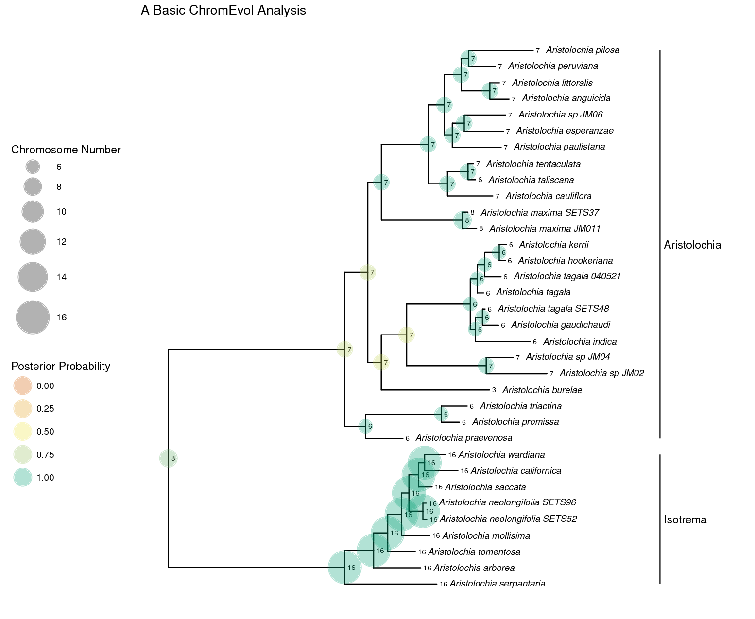
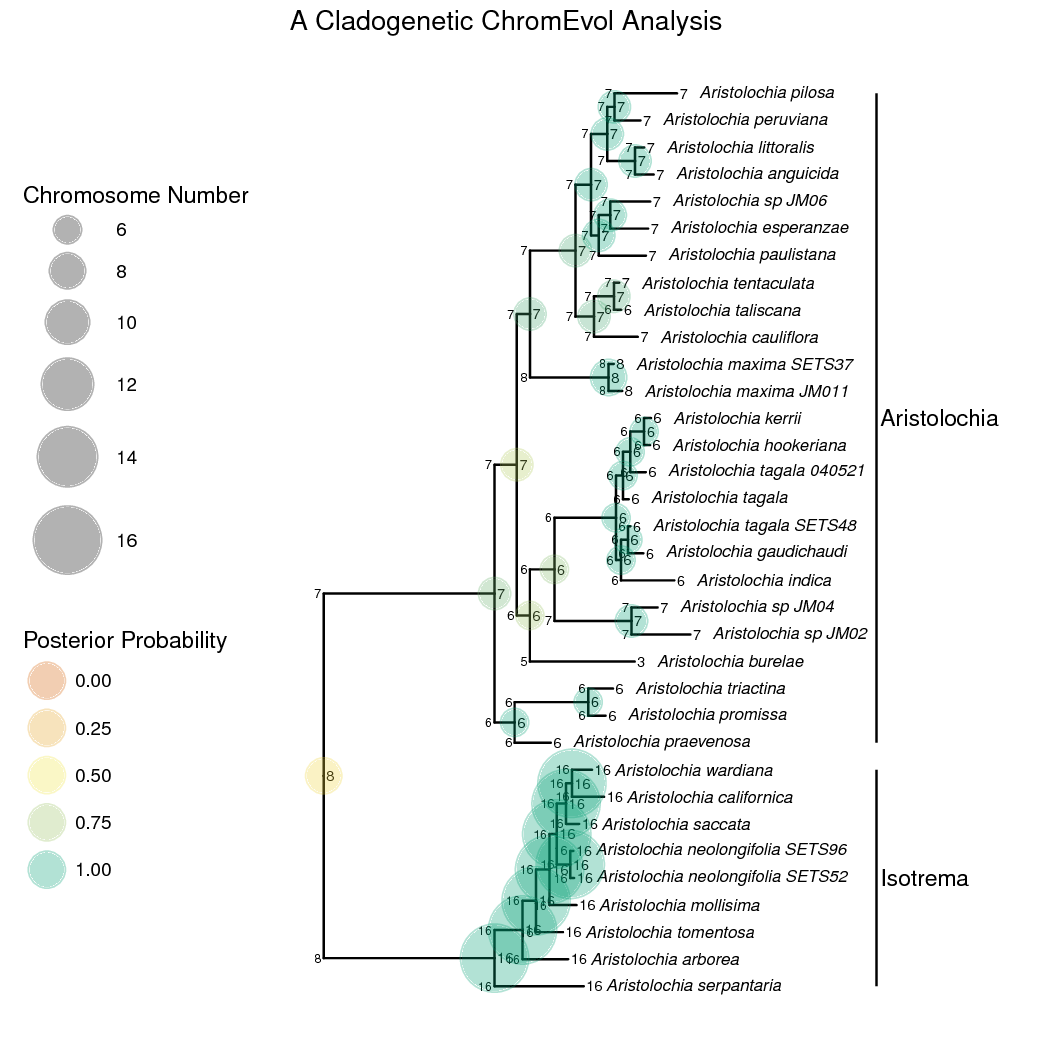
In this example, we will use molecular sequence data and chromosome counts from (missing reference) of the plant genus Aristolochia (commonly called Dutchman’s pipe plants). We will use a simple ChromEvol model to infer rates of chromosome evolution and ancestral chromosome numbers.
Tutorial Format
This tutorial follows a specific format for issuing instructions and information.
All command-line text, including all Rev syntax, are given in
monotype font. Furthermore, blocks of Rev code that are needed to
build the model, specify the analysis, or execute the run are given in
separate shaded boxes. For example, we will instruct you to create a
constant node called example that is equal to 1.0 using the <-
operator like this:
example <- 1.0
Data and Files
On your own computer, create a directory called chromosome_tutorial (or any name you like).
In this directory download and unzip the archive containing the data
files: data.zip.
This will create a folder called data that contains the files
necessary to complete this exercise.
Creating the Rev File
Create a new directory (in chromosome_tutorial) called scripts
. (If you do not have this folder, please refer to the directions in
the section .)
When you execute RevBayes in this exercise, you should do so within
the main directory you created (chromosome_tutorial),
thus, if you are using a Unix-based operating system, we recommend that
you add the RevBayes binary to your path.
For complex models and analyses, it is best to create Rev script files
that will contain all of the model parameters, moves, and functions. In
this first section, you will create a file called from scratch and save
it in the scripts directory.
The full scripts for these examples are also provided for download as
scripts.zip. Please refer to these files to verify or
troubleshoot your own scripts.
Open your text editor and enter the Rev code provided in this section.
Save this Rev file into your scripts directory.
This file will be the one you load into RevBayes to run the analysis.
The file will contain the Rev code to load the data files, set up the
model, run the MCMC analysis, and summarize the results.
Reading in Data
First, we’ll read in the phylogeny. In this example the phylogeny is assumed known. In further examples we’ll jointly estimate chromosome evolution and the phylogeny.
phylogeny <- readBranchLengthTrees("data/aristolochia.tree")[1]
We need to limit the maximum number of chromosomes allowed in our model, so here we use the largest observed chromosome count plus 10. This is an arbitrary limit on the size of the state space that could be increased if necessary.
max_chromo = 26
Now we get the observed chromosome counts from a tab-delimited file.
chromo_data = readCharacterDataDelimited("data/aristolochia_chromosome_counts.tsv", stateLabels=(max_chromo + 1), type="NaturalNumbers", delimiter="\t", header=FALSE)
Finally, we initialize a variable for our vector of moves and monitors.
moves    = VectorMoves()
    monitors = VectorMonitors()
The Chromosome Evolution Model
We’ll use exponential priors with prior mean 0.1 to model the rates of
polyploidy and dysploidy events along the branches of the phylogeny.
gamma is the rate of chromosome gains, delta is the rate of
chromosome losses, and rho is the rate of polyploidization.
gamma ~ dnExponential(10.0)
delta ~ dnExponential(10.0)
rho ~ dnExponential(10.0)
Add MCMC moves for each of the rates.
moves.append( mvScale(gamma, lambda=1, weight=1) )
moves.append( mvScale(delta, lambda=1, weight=1) )
moves.append( mvScale(rho, lambda=1, weight=1) )
Now we create the rate matrix for the chromosome evolution model. Here we will use a simple ChromEvol model that includes only the rate of chromosome gain, loss, and polyploidization.
Q := fnChromosomes(max_chromo, gamma, delta, rho)
Parameters for demi-polyploidization and rate modifiers could also be
added at this step for more complex models. For example, we could have
included the rate of demi-polyploidization eta and rate modifiers like
this:
Q := fnChromosomes(max_chromo, gamma, delta, rho, eta, gamma_l, delta_l)
Here we assume an equal prior probability for the frequency of chromosome numbers at the root of the tree. This does not mean that the frequencies are actually equal, we just give it an equal prior probability. Alternatively, we could have treated the root frequencies as a free variable and estimated them from the observed data. This approach will be illustrated in further examples.
root_frequencies := simplex(rep(1, max_chromo + 1))
Finally, we create the stochastic node for the chromosome evolution continuous-time Markov chain (CTMC). We also clamp the observed chromosome count data to the CTMC.
chromo_ctmc ~ dnPhyloCTMC(Q=Q, tree=phylogeny, rootFreq=root_frequencies, type="NaturalNumbers")
chromo_ctmc.clamp(chromo_data)
All of the components of the model are now specified, so now we wrap it into a single model object.
mymodel = model(phylogeny)
Set Up the MCMC
The next important step for our master Rev file is to specify the MCMC
monitors. For this, we create a vector called monitors that will each
output MCMC samples. First, a screen monitor that will output every 10
iterations:
monitors.append( mnScreen(printgen=10) )
Next, an ancestral state monitor which will sample ancestral states and
write them to a log file. We could additionally use the
mnStochasticCharacterMap monitor to sample stochastic character maps
of chromosome evolution (see the next section for an example).
monitors.append( mnJointConditionalAncestralState(filename="output/ChromEvol_simple_anc_states.log", printgen=10, tree=phylogeny, ctmc=chromo_ctmc, type="NaturalNumbers") )
And another monitor for logging all the model parameters. This will
generate a file that can be opened in Tracerfor checking
MCMC convergence and parameter estimates.
monitors.append( mnModel(filename="output/ChromEvol_simple_model.log", printgen=10) )
Now we set up the MCMC and include code to execute the analysis. In this
example we set the chain length to 200, however for a real analysis
you would want to run many more iterations and check for convergence.
mymcmc = mcmc(mymodel, monitors, moves)
mymcmc.run(200)
Summarize Ancestral States
Now we need to add Rev code that will summarize the sampled ancestral
chromosome numbers. First, read in the ancestral state trace generated
by the ancestral state monitor during the MCMC analysis:
anc_state_trace = readAncestralStateTrace("output/ChromEvol_simple_anc_states.log")
Finally, summarize the values from the traces over the phylogeny. Here
we do a marginal reconstruction of the ancestral states, discarding the
first 25% of samples as burnin. This will produce the file
ChromEvol_simple_final.tree that contains the phylogeny along with
estimated ancestral states. We can use that file with the RevGadgets R
package to generate a plot of the ancestral states.
ancestralStateTree(phylogeny, anc_state_trace, "output/ChromEvol_simple_final.tree", burnin=0.25, reconstruction="marginal")
Note that we could also have calculated joint or conditional ancestral
states instead of (or in addition to) the marginal ancestral states. If
we had sampled stochastic character maps, we would summarize them with
the characterMapTree function.
And now quit RevBayes:
q()
You made it! Be sure to save the file.
Execute the RevBayes Analysis
With all the parameters specified and all analysis components in place,
you are now ready to run your analysis. The Rev scripts you just
created will all be used by RevBayes and loaded in the appropriate
order.
Begin by running the RevBayes executable. In Unix systems, type the following in your terminal (if the RevBayes binary is in your path):
Provided that you started RevBayes from the correct directory
(RB_Chromsome_Evolution_Tutorial) the analysis should now run.
Alternatively, from within RevBayes you could use the source()
function to feed RevBayes your master script file:
source("scripts/ChromEvol_simple.Rev")
This will execute the analysis and you should see output similar to this (though not the exact same values):
When the analysis is complete, RevBayes will quit and you will have a
new directory called output that will contain all of the files you
specified with the monitors.
Plotting the Results
Now we will plot the results of the MCMC analysis using the RevGadgets
R package. Start R and set your working directory to the
RB_Chromsome_Evolution_Tutorial directory. Now run the command to
generate below. There are many options
to customize the look of the plot, for options take a look inside the R
script.
Next Steps
There are many extensions to the basic ChromEvol analysis demonstrated here. In the next section we will look at how to set up more complex chromosome number evolution analyses.
Basic extensions of the ChromEvol model
In this section, we will extend the ChromEvol model in a number of ways. First, we will examine another approach for treating chromosome number root frequencies. This is followed by a brief example applying stochastic character mapping to chromosome evolution models. Then will look at jointly estimating the phylogeny and chromsome evolution, show how to set up a BiChroM analysis, and demonstrate one way to add cladogenetic changes to a chromosome evolution analysis.
Like before, scripts for these examples are also provided in the
scripts.zip file. Please refer to these files to
verify or troubleshoot your own scripts.
Improved root frequencies
In the last example we assumed the frequency of chromosome numbers at the root of the tree were equal. This is equivalent to assigning an extremely informative prior that all root states are equally likely. An alternative approach is to treat the root frequencies as free parameters of the model and estimate them from the observed data. In a series of unpublished simulations performed by the authors this resulted in increased accuracy of ancestral root chromosome numbers estimates.
To use this approach, the root_frequencies parameter must be redefined
as a stochastic node in our graphical model instead of a deterministic
node. Remove the following line from your Rev script:
root_frequencies := simplex(rep(1, max_chromo + 1))
We will instead use an uninformative flat Dirichlet prior for the root frequencies. First, we create a vector to hold the concentration parameters for the Dirichlet distribution. Here we set all concentration parameters to 1, which results in all sets of probabilities being equally likely. We then pass the vector of concentration parameters into the Dirichlet distribution and create the stochastic node representing root frequencies.
root_frequencies_prior <- rep(1, max_chromo + 1)
root_frequencies ~ dnDirichlet(root_frequencies_prior)
Next, we must specify MCMC moves for the root frequencies. When the
maximum number of chromosomes is high these parameters can have
difficulty converging. Therefore, we use two different MCMC moves. The
first is Beta Simplex move, which selects one element of the
root_frequencies vector and proposes a new value for it drawn from a
Beta distribution. The second is Element Swap Simplex move, which
selects two elements of the root_frequencies vector and simply swaps
their values.
moves.append( mvBetaSimplex(root_frequencies, alpha=0.5, weight=10)
moves.append( mvElementSwapSimplex(root_frequencies, weight=10)
You can experiment with different weights for each MCMC move.
Make the modifications to the root frequencies in the script
ChromoSSE_simple.Rev and run the analysis again? What are the
estimates of the root frequency (you can see this by looking at the
output in Tracer)? Do the estimated ancestral states
change?
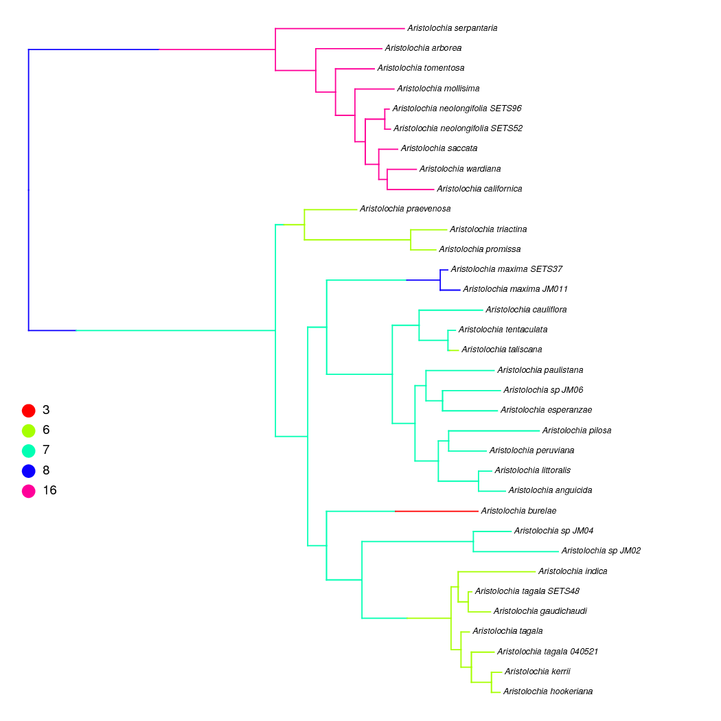
Stochastic character mapping of chromosome evolution
In RevBayes both ancestral states and stochastic character maps can be sampled from continuous-time Markov chain (CTMC) and state-dependent speciation and extinction (SSE) models of character evolution. Stochastic character maps show the timing and number of transitions along the branches of the phylogeny, so they can be particularly useful for chromosome evolution estimates where the timing of, for example, whole genome duplication events might be of interest. This example is performed on a non-ultrametric tree, but the same analysis could be performed on time-calibrated trees.
We have already shown how to sample ancestral states above, and here we
show the few extra lines of Rev code needed to sample stochastic
character maps. Stochastic character maps are drawn during the MCMC, so
we need to include the mnStochasticCharacterMap monitor.
monitors.append( mnStochasticCharacterMap(ctmc=chromo_ctmc, filename="output/ChromEvol_maps.log", printgen=10) )
This monitor will create the output/ChromEvol_maps.log file. Just like
the other log files, each row in this file represents a different sample
from the MCMC. Each column in the file, though, is the character history
for a different node in the phylogeny. The last column of the file is
the full stochastic character map of the entire tree in SIMMAP
(Bollback 2006) format. These can be plotted using the
phytools R package (Revell 2012).
After the MCMC simulation, we can calculate the maximum a posteriori marginal, joint, or conditional character history. This process is similar to the ancestral state summaries. First we read in the stochastic character map trace.
anc_state_trace = readAncestralStateTrace("output/ChromEvol_maps.log")
Then we use the characterMapTree function. This generates two SIMMAP
formatted files: 1) the maximum a posteriori character history, and 2)
the posterior probabilities of the entire character history.
characterMapTree(phylogeny, anc_state_trace, character_file="output/character.tree", posterior_file="output/posterior.tree", burnin=5, reconstruction="marginal")
is an example stochastic character map of our Aristolochia analysis plotted using phytools.
Copy the script ChromoSSE_simple.Rev and add stochastic character
mapping monitor. Then, run the analysis and use the script
plot_simmap.R to visualize the character mappings.
Joint estimation of phylogeny and chromosome evolution
In RevBayes the chromosome evolution models can be used jointly with a model of molecular evolution enabling joint inference of the phylogeny and chromosome number evolution. This enables the chromosome number analysis to take into account phylogenetic uncertainty and allows the chromosome numbers to help inform the phylogeny.
Setting up a model that jointly infers chromosome evolution and
phylogeny requires mostly combining elements covered in the Molecular
Models of Character Evolution tutorial with what has already been
covered in Section [sec:chromo_basic_analysis] of this tutorial. We
will not repeat how to set up the chromosome model component, but we’ll
step through what must be added to the example in the section
above. Furthermore, we have provided a
full working example script scripts/ChromEvol_joint.Rev.
Reading in Molecular Data and Setting Clade Constraints
The first major difference from the basic ChromEvol example shown above is that we must additionally read in molecular sequence data:
dna_seq = readDiscreteCharacterData("data/aristolochia_matK.fasta")
We will need some useful information about this data as well:
n_species = dna_seq.ntaxa()
n_sites = dna_seq.nchar()
taxa = dna_seq.names()
n_branches = 2 * n_species - 2
Since we want to jointly infer ancestral states, we need to set an a priori rooting constraint on our phylogeny. So here we set an ingroup and outgroup.
outgroup = ["Aristolochia_serpantaria", "Aristolochia_arborea",
            "Aristolochia_wardiana", "Aristolochia_californica",
            "Aristolochia_saccata", "Aristolochia_mollisima",
            "Aristolochia_tomentosa", "Aristolochia_neolongifolia_SETS52",
            "Aristolochia_neolongifolia_SETS96"]
Here we loop through each taxon and if it is not present in the outgroup defined above we add it to the ingroup.
i = 1
for (j in 1:taxa.size()) {
    found = false
    for (k in 1:outgroup.size()) {
        if (outgroup[k] == taxa[j].getSpeciesName()) {
            found = true
            break
        }
    }
    if (found == false) {
        ingroup[i] = taxa[j].getSpeciesName()
        i += 1
    }
}
And now we make the vector of clade objects to constrain our tree topology.
clade_ingroup = clade(ingroup)
clade_outgroup = clade(outgroup)
clade_constraints = [clade_ingroup, clade_outgroup]
Tree Model
We will specify a uniform prior on the tree topology, and add a MCMC move on the topology.
topology ~ dnUniformTopology(taxa=taxa, constraints=clade_constraints, rooted=TRUE)
moves.append( mvNNI(topology, weight=10.0) )
Next, we create a stochastic node for each branch length. Each branch length prior will have an exponential distribution with rate 1.0. We’ll also add a simple scaling move for each branch length.
for (i in 1:n_branches) {
    br_lens[i] ~ dnExponential(10.0)
    moves.append( mvScale(br_lens[i], lambda=2, weight=1)
}
Finally, build the tree by combining the topology with the branch lengths.
phylogeny := treeAssembly(topology, br_lens)
Molecular Substitution Model
We’ll specify the GTR substitution model applied uniformly to all sites. Use a flat Dirichlet prior for the exchange rates.
er_prior <- v(1,1,1,1,1,1)
er ~ dnDirichlet(er_prior)
moves.append( mvSimplexElementScale(er, alpha=10, weight=3) )
And also a flat Dirichlet prior for the stationary base frequencies.
pi_prior <- v(1,1,1,1)
pi ~ dnDirichlet(pi_prior)
moves.append( mvSimplexElementScale(pi, alpha=10, weight=2) )
Now create a deterministic variable for the nucleotide substitution rate matrix.
Q_mol := fnGTR(er, pi)
Create a stochastic node for the sequence evolution continuous-time Markov chain (CTMC) and clamp the sequence data. Note we should have two CTMC objects in this model: one for the model of molecular evolution and one for the model of chromosome evolution.
dna_ctmc ~ dnPhyloCTMC(tree=phylogeny, Q=Q_mol, branchRates=1.0, type="DNA")
dna_ctmc.clamp(dna_seq)
MCMC and Summarizing Results
We set up the MCMC just as before, except here we need to add a file monitor to store the sampled trees.
monitors.append( mnFile(filename="output/ChromEvol_joint.trees", printgen=10, phylogeny) )
Summarizing the results of the MCMC analysis are a little different. First we will calculate the maximum a posteriori (MAP) tree.
treetrace = readAncestralStateTreeTrace("output/ChromEvol_joint.trees", treetype="non-clock")
map_tree = mapTree(treetrace, "output/ChromEvol_joint_map.tree")
Now we’ll summarize the ancestral chromosome numbers over the MAP tree. Read in the ancestral state trace:
anc_state_trace = readAncestralStateTrace("output/ChromEvol_joint_states.log")
Finally, calculate the marginal ancestral states from the traces over
the MAP tree. Note that this time we have to pass both the tree trace
and the ancestral state trace to the ancestralStateTree function.
Since we sampled a joint distribution of ancestral state histories and
trees, we sampled some ancestral states for nodes that do not exist in
the MAP tree. Therefore the ancestral state probabilities being
calculated for the MAP tree are conditional to the probability of the
node existing.
ancestralStateTree(map_tree, anc_state_trace, treetrace, "output/ChromEvol_joint_final.tree" burnin=0.25, reconstruction="marginal")
Like before, we can plot the results using the RevGadgets R package
using the script plot_ChromEvol_joint.R.
Association chromosome evolution with phenotype (BiChroM)
We may be interested in testing whether the rates of chromosome number evolution are associated with a certain phenotype. Here we set up a binary phenotypic character and estimate separate rates of chromosome evolution for each state of the phenotype. We’ll use a model that describes the joint evolution of both the phenotypic character and chromosome evolution. This model (BiChroM) was introduced in (missing reference). In RevBayes, the BiChroM model can easily be extended to multistate phenotypes and/or hidden states, plus cladogenetic changes could be incorporated into the model.
In this example we will again use chromosome count data from (missing reference) for the plant genus Aristolochia. For the phenotype we will examine gynostemium morphology. Aristolochia flowers have an extensively modified perianth that traps and eventually releases pollinators to ensure cross pollination (this is why the flowers resemble pipes and are commonly called Dutchman’s pipes). The gynostemium is a reproductive organ found only in Aristolchiaceae and Orchids that consists of fused stamens and pistil that pollinators must interact with during pollination. The subgenus Isotrema has highly reduced three-lobed gynostemium. Other members of Aristolochia have gynostemium subdivided into 5 to 24 lobes. We’ll test for an association of this phenotype with changes in the rates of chromosome evolution.
- phenotype state 0 = 3 lobed gynostemium
- phenotype state 1 = 5 to 24 lobed gynostemium
Much of this exercise is a repeat of what was already covered in section ,
so we will only touch on the model
components that are different. We have provided a full working example
script scripts/BiChroM.Rev. In this example the phylogeny is assumed
known, however one could combine this with the exercise above to jointly
infer the phylogeny.
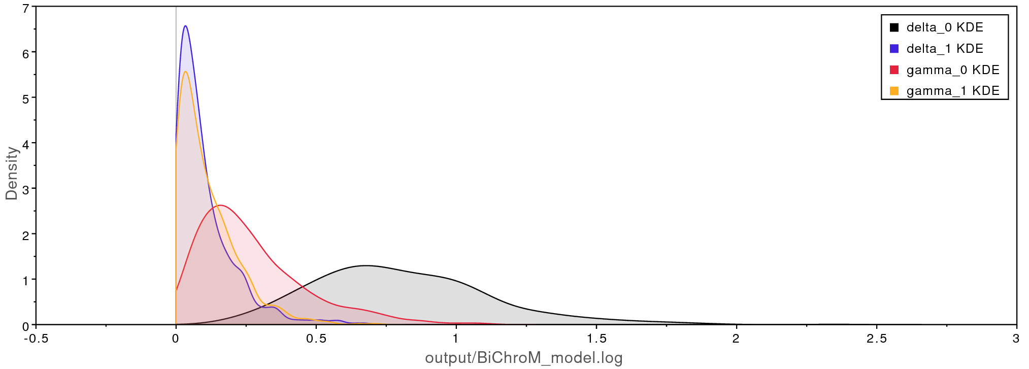
.log
files when loaded into Tracer. The rates of chromosome
gains (gamma) and losses (delta) are higher for Aristolochia
lineages with complex gynostemium subdivided into 5 to 24 lobes (state
0) compared to lineages with simple 3 lobed gynostemium (state 1).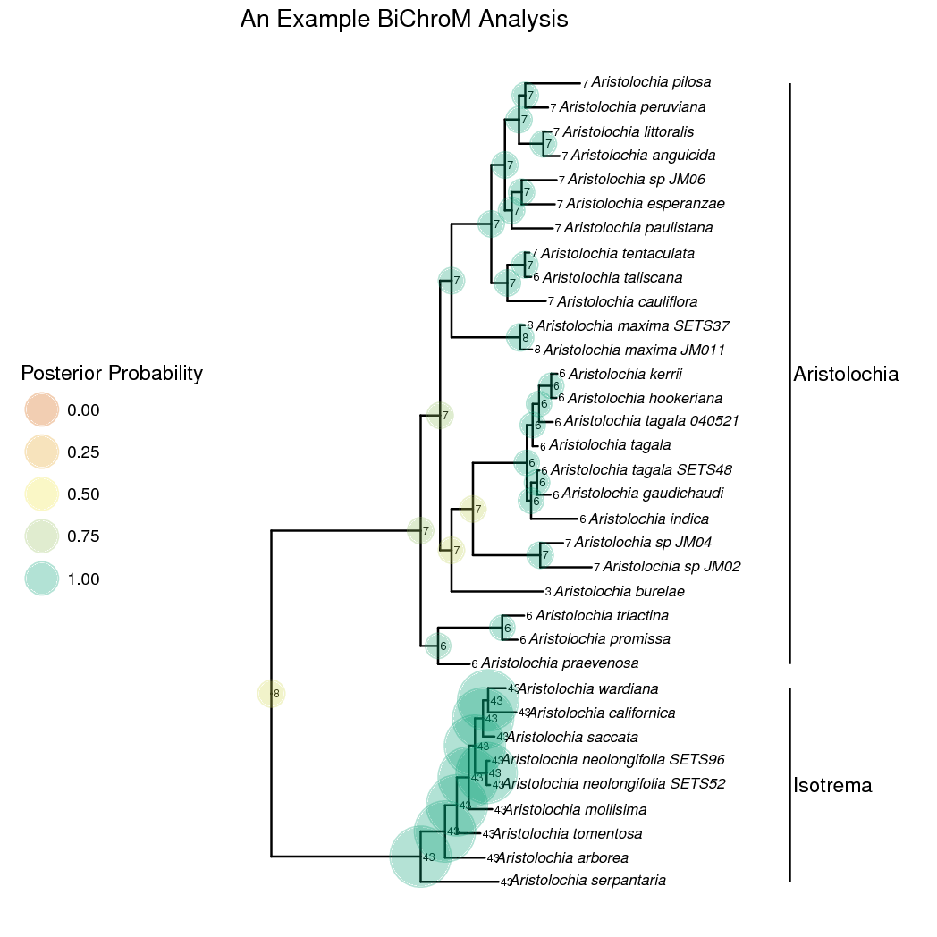
Setting up the BiChroM model
The first step will be to read in the observed data. This is done as
before, with the exception that the data is set up a bit differently.
The data matrix must now represent both the observed chromosome counts
and the observed phenotype. So in this file states 1-26 represent the
haploid number $n$ of chromosome for lineages with gynostemium
subdivided in 5 to 24 lobes, and states 27-52 represent the haploid
number $n + 27$ for lineages with simple 3 lobed gynostemium. Note the
stateLabels argument must now be set to 2 times the maximum number of
chromosomes.
chromo_data = readCharacterDataDelimited("data/aristolochia_bichrom_counts.tsv", stateLabels=2*(max_chromo + 1), type="NaturalNumbers", delimiter="\t", headers=FALSE)
Like before, we’ll use exponential priors to model the rates of polyploidy and dysploidy events along the branches of the phylogeny. However, here we set up two rate parameters for each type of chromosome change – one for phenotype state 0 and one for phenotype state 1.
gamma_0 ~ dnExponential(10.0)
gamma_1 ~ dnExponential(10.0)
delta_0 ~ dnExponential(10.0)
delta_1 ~ dnExponential(10.0)
rho_0 ~ dnExponential(10.0)
rho_1 ~ dnExponential(10.0)
Add MCMC moves for each of the rates.
moves.append( mvScale(gamma_0, lambda=1, weight=1) )
moves.append( mvScale(delta_0, lambda=1, weight=1) )
moves.append( mvScale(rho_0, lambda=1, weight=1) )
moves.append( mvScale(gamma_1, lambda=1, weight=1) )
moves.append( mvScale(delta_1, lambda=1, weight=1) )
moves.append( mvScale(rho_1, lambda=1, weight=1) )
Now we create the rate matrix for the chromosome evolution model. We will set up two rate matrices, one for each phenotype state.
Q_0 := fnChromosomes(max_chromo, gamma_0, delta_0, rho_0)
Q_1 := fnChromosomes(max_chromo, gamma_1, delta_1, rho_1)
Again, we could have include the rate of demi-polyploidization eta and
rate modifiers like this:
Q_0 := fnChromosomes(max_chromo, gamma_0, delta_0, rho_0, eta_0, gamma_l_0, delta_l_0)
Q_1 := fnChromosomes(max_chromo, gamma_1, delta_1, rho_1, eta_1, gamma_l_1, delta_l_1)
Now we create the rates of transitioning between phenotype states. Any model could be used (all rates equal models, Dollo models, etc.) but here we estimate a different rate for each transition between states 0 and 1.
q_01 ~ dnExponential(10.0)
q_10 ~ dnExponential(10.0)
moves.append( mvScale(q_01, lambda=1, weight=1) )
moves.append( mvScale(q_10, lambda=1, weight=1) )
And finally we create the transition rate matrix Q_b for the joint
model of phenotypic and chromosome evolution. First we will initialize
the matrix with all zeros:
s = Q_0[1].size()
for (i in 1:(2 * s)) {
    for (j in 1:(2 * s)) {
        Q[i][j] := 0.0
    }
}
And now we populate the matrix with the transition rates.
for (i in 1:(2 * s)) {
    for (j in 1:(2 * s)) {
        if (i <= s) {
            if (j <= s) {
                if (i != j) {
                    # chromosome changes within phenotype state 0
                    Q[i][j] := abs(Q_0[i][j])
                }
            } else {
                if (i == (j - s)) {
                    # transition from phenotype state 0 to 1
                    Q[i][j] := q_01
                }
            }
        } else {
            if (j <= s) {
                if (i == (j + s)) {
                    # transition from phenotype state 1 to 0
                    Q[i][j] := q_10
                }
            } else {
                if (i != j) {
                    # chromosome changes within phenotype state 1
                    k = i - s
                    l = j - s
                    Q[i][j] := abs(Q_1[k][l])
                }
            }
        }
    }
}
Q_b := fnFreeK(Q, rescaled=false)
The rest of the analysis is essentially the same as in section
. Just make sure to pass the Q_b matrix
into the CTMC object.
BiChroM Analysis Results
In the rates of chromosome gains and losses for each of the phenotype states are plotted. Aristolochia lineages with complex gynostemium subdivided into many lobes have higher rates of dysploid changes than lineages with simple 3-lobed gynostemium. In the marginal maximum a posteriori estimates of ancestral chromosome number and gynostemium morphology are plotted. From this we can see that an evolutionary reduction occured on the lineage leading to the Isotreme clade. The common ancestor for all Aristolochia is inferred to have complex many lobed gynostemium which was reduced to a more simple 3-lobed form in Isotrema.
Incorporating cladogenetic and anagenetic chromosome change
Changes in chromosome number can increase reproductive isolation and may drive the diversification of some lineages (missing reference). To test for the association of chromosome changes with speciation we must extend our models to incorporate cladogenetic changes [for details see Freyman and Höhna (2018)]. Cladogenetic changes are changes that occur only at lineage splitting events. All models of chromosome evolution that we have examined so far model only anagenetic changes, i.e., changes that occur within a lineage.
We introduce here a simple model of cladogenetic change that handles cladogenetic events similarly to the widely used Dispersal-Extinction-Cladogenesis (missing reference) models of biogeographic range evolution. A major limitation of such models is that they only model cladogenetic changes at the observed speciation events on the phylogeny. Many other unobserved speciation events likely occurred, but are not present in the reconstructed phylogeny due to incomplete taxon sampling and lineages going extinct. This can bias the relative rates of anagenetic and cladogenetic change. In section we will introduce the ChromoSSE model, which removes this bias by explicitly modeling unobserved speciation events but at the cost of additional model complexity.
Much of this exercise is a repeat of what was already covered in section
, so we will only touch on the model
components that must be changed to incorporate cladogenetic changes. We
have provided a full working example script
scripts/ChromEvol_clado.Rev
A Simple Cladogenetic Model
The anagenetic transition rate matrix should be set up just as before. The cladogenetic changes, though, are modeled as a vector of probabilities that sum up to 1 (a simplex). Each element of the vector is the probability of a certain type of cladogenetic event occurring. To set this up, we’ll first draw a ‘weight’ for each type of cladogenetic event from an exponential distribution. To keep the example simple we are excluding cladogenetic demi-polyploidization. We then pass each ‘weight’ into a simplex to create the vector of probabilities.
clado_no_change_pr ~ dnExponential(10.0)
clado_fission_pr ~ dnExponential(10.0)
clado_fusion_pr ~ dnExponential(10.0)
clado_polyploid_pr ~ dnExponential(10.0)
clado_demipoly_pr <- 0.0
clado_type := simplex([clado_no_change_pr, clado_fission_pr, clado_fusion_pr, clado_polyploid_pr, clado_demipoly_pr])
The function fnChromosomesCladoProbs produces a matrix of cladogenetic
probabilities. This is a very large and sparse 3 dimensional matrix that
contains the transition probabilities of every possible state of the
parent lineage transitioning to every possible combination of states of
the two daughter lineages.
clado_prob := fnChromosomesCladoProbs(clado_type, max_chromo)
We can’t forget to add moves for each cladogenetic event:
moves.append( mvScale(clado_no_change_pr, lambda=1.0, weight=2) )
moves.append( mvScale(clado_fission_pr, lambda=1.0, weight=2) )
moves.append( mvScale(clado_fusion_pr, lambda=1.0, weight=2) )
moves.append( mvScale(clado_polyploid_pr, lambda=1.0, weight=2) )
Now we can create the cladogenetic CTMC model. We must pass in both the
Q matrix that represents the anagenetic changes, and the clado_probs
matrix that represents the cladogenetic changes.
chromo_ctmc ~ dnPhyloCTMCClado(Q=Q, tree=phylogeny, cladoProbs=clado_prob, rootFrequencies=root_frequencies, type="NaturalNumbers", nSites=1)
Most of the rest of the analysis is the same. For the ancestral state
monitor we want to be sure to specify withStartState=true so that we
sample the states both at start and end of each branch. This enables us
to reconstruct cladogenetic events.
monitors.append( mnJointConditionalAncestralState(filename="output/ChromEvol_clado_anc_states.log", printgen=10, tree=phylogeny, ctmc=chromo_ctmc, withStartStates=true, type="NaturalNumbers") )
When summarizing the ancestral state results we also want to specify
include_start_states=true so that we summarize the cladogenetic
changes.
ancestralStateTree(phylogeny, anc_state_trace, "output/ChromEvol_clado_final.tree", include_start_states=true, burnin=0.25, reconstruction="marginal")
And that’s it! shows the ancestral state estimates plotted on the tree. The start states of each lineage (the state after cladogenesis) are plotted on the ‘shoulders’ of each lineage. You may want to try stochastic character mapping for a different and possibly better visualization of cladogenetic and anagenetic changes.
Overview of the ChromoSSE model
A major challenge for all phylogenetic models of cladogenetic character change is accounting for unobserved speciation events due to lineages going extinct and not leaving any extant descendants (Bokma 2002), or due to incomplete sampling of lineages in the present. Teasing apart the phylogenetic signal for cladogenetic and anagenetic processes given unobserved speciation events is a major difficulty, and using a naive approach that does not account for unobserved speciation (like the ones discussed earlier in section ) can bias the relative rates of cladogenetic and anagenetic change. The Cladogenetic State change Speciation and Extinction (ClaSSE) model (Goldberg and Igić 2012), on the other hand, reduces this bias by explicitly incorporating unobserved speciation events. This is achieved by jointly modeling both character evolution and the phylogenetic birth-death process. Not only does the ClaSSE framework enable the modeling of unobserved speciation, but it also provides an easily extensible framework for testing state-dependent speciation and extinction rates.
The ChromoSSE model (Freyman and Höhna 2018) is a special case of the ClaSSE model that models chromosome changes. Compared to the previously discussed CTMC models of chromosome evolution, SSE models require additional complexity since they must also model the speciation and extinction process. Simple extensions to the ChromoSSE model will enable explicit tests of different extinction rates for polyploid and diploid lineages, and testing different rates of chromosome speciation associated with phenotypes or habitat.
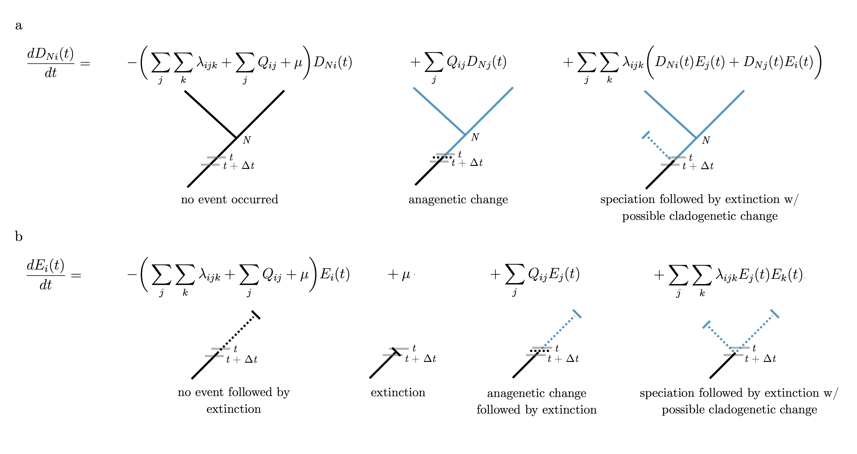
The ChromoSSE likelihood calculation
All the previous models of chromosome number evolution discussed in the tutorial used the standard pruning algorithm (Felsenstein 1981) to calculate the likelihood of chromosome evolution over the phylogeny. For the ChromoSSE model we must use a different approach; here the likelihood is calculated using a set of ordinary differential equations similar to the Binary State Speciation and Extinction (BiSSE) model (Maddison et al. 2007). The BiSSE model was extended to incorporate cladogenetic changes by Goldberg and Igić (2012). Following Goldberg and Igić (2012), we define $D_{Ni}(t)$ as the probability that a lineage with chromosome number $i$ at time $t$ evolves into the observed clade $N$. We let $E_i(t)$ be the probability that a lineage with chromosome number $i$ at time $t$ goes extinct before the present, or is not sampled at the present. These two differential equations are shown and explained in . However, unlike the full ClaSSE model the extinction rate $\mu$ does not depend on the chromosome number $i$ of the lineage. This can easily be modified in RevBayes to allow for different speciation and/or extinction rates depending on ploidy or other character states.
Next Steps
In the next section we’ll set up and run a RevBayes analysis using the ChromoSSE model of cladogenetic and anagenetic chromosome evolution.
A simple ChromoSSE analysis
In this example, we will again use molecular sequence data and chromosome counts from (missing reference) of the plant genus Aristolochia. We will use a ChromoSSE model to infer rates of chromosome evolution and ancestral chromosome numbers. For more complex examples utilizing ChromoSSE with Bayesian model averaging and reversible-jump MCMC, see the scripts and explanations at https://github.com/wf8/chromosse.
Like in previous examples, we will here only highlight the major
differences between a ChromoSSE analysis and the ChromEvol analysis set
up in section . The full script to run
this ChromoSSE example is provided in the file
scripts/ChromoSSE_simple.Rev.
The model: a joint model of the tree and chromosome evolution
A major difference between the previously discussed models of chromosome number evolution and ChromoSSE is that ChromoSSE jointly describes the evolution of chromosome numbers and the tree. Since ChromoSSE assumes the tree is generated via a birth-death process you should use an ultrametric tree or time-calibrated tree. The tree may contain lineages that went extinct before the present, but the branch lengths should be in units of time, as opposed to units of substitutions per site. So here we will swap out the tree used in previous examples for a tree that was time-calibrated. The estimated rates of chromosome evolution will have the same unit of time as the branch lengths of our tree. In this example the node ages are relative, but you could use a fossil-calibrated tree with absolute ages if you wanted rates of chromosome change in units of millions of years.
phylogeny <- readTrees("data/aristolochia-bd.tree")[1]
Anagenetic Changes
The anagenetic part of the chromosome number evolution model involves
populating the Q transition rate matrix with the rates of anagenetic
chromosome number changes. This is set up exactly the same as in the
ChromEvol analyses before.
Cladogenetic Changes
At each lineage splitting event a number of different types of cladogenetic events could occur, including no change in chromosome numbers, a dysploid gain or loss in a single daughter lineage, or a change in ploidy in a single daughter lineage. So we must set up a separate speciation rate for each type of cladogenetic event.
For each speciation rate, we will use an exponential prior with the mean value set to $r$, where $r$ is an approximation of the net diversification rate. We calculate this approximation using $E(N_t) = N_0 e^{rt}$, which describes the expected number of species $N_t$ at time $t$ under a constant rate birth-death process where $N_0$ is the number of species at $t=0$ (missing reference). The equation can be rearranged to arrive at $r = ( \ln(N_t) - \ln(N_0) ) / t$.
taxa <- phylogeny.taxa()
speciation_mean <- ln( taxa.size() ) / phylogeny.rootAge()
speciation_pr <- 1 / speciation_mean
Each cladogenetic event type is assigned its own speciation rate. We set the rate of demi-polyploidization to 0.0 for simplicity.
clado_no_change ~ dnExponential(speciation_pr)
clado_fission ~ dnExponential(speciation_pr)
clado_fusion ~ dnExponential(speciation_pr)
clado_polyploid ~ dnExponential(speciation_pr)
clado_demipoly <- 0.0
Like usual, we must add MCMC moves for the speciation rates.
moves.append( mvScale(clado_no_change, lambda=5.0, weight=1) )
moves.append( mvScale(clado_fission, lambda=5.0, weight=1) )
moves.append( mvScale(clado_fusion, lambda=5.0, weight=1) )
moves.append( mvScale(clado_polyploid, lambda=5.0, weight=1) )
We next create a vector to hold the speciation rates, and also create a
deterministic node total_speciation which will be a convenient way to
monitor the total speciation rate of the birth-death process.
speciation_rates := [clado_no_change, clado_fission, clado_fusion, clado_polyploid, clado_demipoly]
total_speciation := sum(speciation_rates)
Finally, we map the speciation rates to the chromosome cladogenetic
events. The function fnChromosomesCladoEventsBD produces a matrix of
speciation rates. This is a very large and sparse 3 dimensional matrix
that contains the speciation rates for all possible cladogenetic events.
It contains the speciation rate for every possible state of the parent
lineage transitioning to every possible combination of states of the two
daughter lineages.
clado_matrix := fnChromosomesCladoEventsBD(speciation_rates, max_chromo)
Extinction Rate
Next, we create a stochastic variable to represent the relative-extinction rate. Here, we define relative-extinction as extinction divided by speciation, so we use a uniform prior on the interval ${0,1}$.
rel_extinction ~ dnUniform(0, 1.0)
rel_extinction(0.4)
moves.append( mvScale(rel_extinction, lambda=5.0, weight=3.0) )
We then make a vector of extinction rates for each state. In the basic ChromoSSE model we assume all chromosome numbers have the same extinction rate.
for (i in 1:(max_chromo + 1)) {
    extinction[i] := rel_extinction * total_speciation
}
The State-Dependent Speciation and Extinction Model
We are now nearly ready to create the stochastic node that represents the state-dependent speciation and extinction process. First, though, we must set the probability of sampling species at the present. We artificially use 1.0 here, but you should experiment with more realistic settings as this will affect the overall speciation and extinction rates estimated.
rho_bd <- 1.0
Now we construct a variable that describes the evolution of both the
tree and chromosome numbers drawn from a cladogenetic state-dependent
birth-death process. The dnCDBDP distribution is named for a
character-dependent birth-death process, which is another
name for a state-dependent speciation and extinction
process.
chromo_bdp ~ dnCDBDP( rootAge            = phylogeny.rootAge(),
                      cladoEventMap      = clado_matrix,
                      extinctionRates    = extinction,
                      Q                  = Q,
                      pi                 = root_frequencies,
                      rho                = rho_bd )
Since ChromoSSE is a joint model of both the tree and the chromosome numbers, we must of course clamp both the observed tree and the chromosome count data.
chromo_bdp.clamp(phylogeny)
chromo_bdp.clampCharData(chromo_data)
Finishing the ChromoSSE Analysis
The rest of the analysis is nearly identical to the other examples we
have worked through, except for one detail when setting up the ancestral
state monitor. Now we must specify that we are using a state-dependent
speciation and extinction process (as mentioned above this is also
called a character-dependent birth-death process, or cdbdp) instead of
a continuous-time Markov process (ctmc) like we use before.
monitors.append( mnJointConditionalAncestralState(filename="output/ChromoSSE_anc_states.log", printgen=10, tree=phylogeny, cdbdp=chromo_bdp, withStartStates=true, type="NaturalNumbers") )
And that’s it! The results can be plotted using the same R script demonstrated before to plot the cladogenetic ChromEvol analysis.
- Bokma F. 2002. Detection of punctuated equilibrium from molecular phylogenies. Journal of Evolutionary Biology. 15:1048–1056. 10.1046/j.1420-9101.2002.00458.x
- Bollback J.P. 2006. SIMMAP: stochastic character mapping of discrete traits on phylogenies. BMC bioinformatics. 7:88.
- Felsenstein J. 1981. Evolutionary Trees from DNA Sequences: a Maximum Likelihood Approach. Journal of Molecular Evolution. 17:368–376. 10.1007/BF01734359
- Freyman W.A., Höhna S. 2018. Cladogenetic and anagenetic models of chromosome number evolution: a Bayesian model averaging approach. Systematic Biology. 67:1995–215.
- Goldberg E.E., Igić B. 2012. Tempo and Mode in Plant Breeding System Evolution. Evolution. 66:3701–3709. 10.1111/j.1558-5646.2012.01730.x
- Maddison W.P., Midford P.E., Otto S.P. 2007. Estimating a binary character’s effect on speciation and extinction. Systematic Biology. 56:701. 10.1080/10635150701607033
- Revell L.J. 2012. phytools: an R package for phylogenetic comparative biology (and other things). Methods in Ecology and Evolution.:217–223.