Skyline Plots
Skyline Plots are models for how population size changes through time.
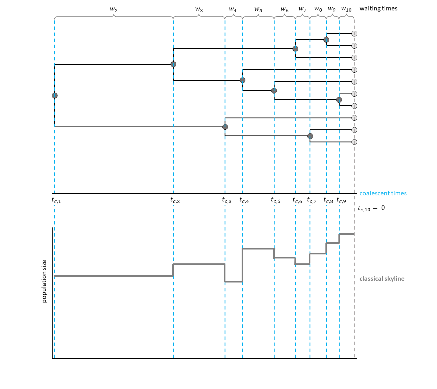
The classical skyline plot (Pybus et al. 2000) provided the first implementation of this idea.
For each interval between two coalescent events, an effective population size was estimated.
This led to a plot looking very similar to a skyline, thus giving the method its name (see for a hypothetical example).
The generalized skyline plot (Strimmer and Pybus 2001) aimed at reducing the noise from analyzing every single interval by grouping several coalescent events into one interval.
This created a smoother curve.
First, these models were used for maximum likelihood (ML) estimation of population sizes through time.
By now, several extensions allowing for Bayesian estimation have been published (see for example Drummond et al. (2005), Heled and Drummond (2008), Minin et al. (2008)).
In RevBayes, a Skyline plot method is implemented with constant or linear population size intervals.
The length of the skyline intervals can either be defined by a specific number of intervals ending at coalescent events, or alternatively be chosen individually without depending on the coalescent events.
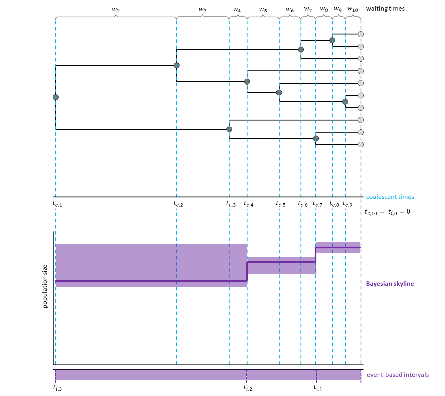
In this exercise, each interval will group five coalescent events.
Have a look at , for a hypothetical example with three events per interval.
Likelihood Calculation
We assume that the phylogeny of the samples is known. There are $n$ samples, with $k$ active lineages at the current point in time $t$. Time starts at $t = 0$. The waiting times between coalescent events $w_k$ are exponentially distributed with rate $c = \frac{k (k-1)}{2N_e(t)}$ with $N_e$ being the population size.
The likelihood for a given piecewise-constant population size trajectory is computed as the product of the probability density functions of the coalescent waiting times, which are calculated as follows:
\[p(w_k | t_{c,k}) = \frac{k (k -1)}{2N_e(t_{c,k} + w_k)} exp \left[ \int_{t_{c,k}}^{t_{c,k}+w_k} \frac{k (k -1)}{2N_e(t)} dt \right]\]Each $t_{c,k}$ is the beginning of the respective kth coalescent interval. The waiting times $w_k$ refer to the waiting time starting when there are $k$ active lineages.
Inference Example
For your info
The entire process of the skyline estimation can be executed by using the mcmc_isochronous_Skyline.Rev script that you can download on the left side of the page. Save it in your scripts directory. You can type the following command into
RevBayes:source("scripts/mcmc_isochronous_Skyline.Rev")We will walk you through the script in the following section.
We will mainly highlight the parts of the script that change compared to the constant coalescent model.
Read the data
Read in the data as described in the first exercise.
The Skyline Model
For the skyline model, you need to decide on the number of intervals. In this case, we would like to have five coalescent events per interval, so we divide the number of coalescent events by five. With $n$ taxa, we expect $(n-1)$ coalescent events, until there is only one lineage left.
NUM_INTERVALS = ceil((n_taxa - 1) / 5)
For each interval, a population size will be estimated. Choose a prior and add a move for each population size. In the following loop, we also set the number of coalescent events per interval by dividing the number of coalescent events by the number of intervals. Remember that we chose the number of intervals based on our wish to have $5$ events per interval.
for (i in 1:NUM_INTERVALS) {

    pop_size[i] ~ dnUniform(0,1E6)
    pop_size[i].setValue(100000)
    moves.append( mvScale(pop_size[i], lambda=0.1, tune=true, weight=2.0) )
    num_events[i] <- ceil( (n_taxa-1) / NUM_INTERVALS )

}
The Tree
Now, we will instantiate the stochastic node for the tree.
The Skyline version of the Coalescent distribution function dnCoalescentSkyline takes the vector of population sizes and the taxa as input.
By chosing methods="events", the interval lengths will be chosen based on the number of events and we have to add the number of coalescent events to the input.
psi ~ dnCoalescentSkyline(theta=pop_size, events_per_interval=num_events, method="events", taxa=taxa)
For later plotting and analyzing the population size curve, we need to retrieve the resulting interval times.
interval_times := psi.getIntervalAges()
For this analysis, we constrain the root age as before and add the same moves for the tree.
Substitution Model and other parameters
This part is also taken from the constant coalescent exercise.
Finalize and run the analysis
Finally, we need to wrap our model as before. We add the monitors and then run the MCMC. Here, an additional monitor is added for the interval times.
monitors.append( mnModel(filename="output/horses_iso_Skyline.log",printgen=THINNING) )
monitors.append( mnFile(filename="output/horses_iso_Skyline.trees",psi,printgen=THINNING) )
monitors.append( mnFile(filename="output/horses_iso_Skyline_NEs.log",pop_size,printgen=THINNING) )
monitors.append( mnFile(filename="output/horses_iso_Skyline_times.log",interval_times,printgen=THINNING) )
monitors.append( mnScreen(pop_size, root_age, printgen=100) )
Results
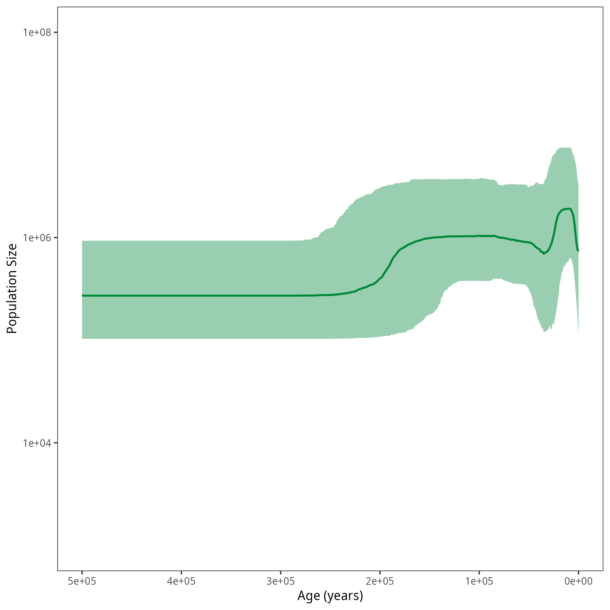
After running your analysis, you can plot the results again using the R package RevGadgets.
library(RevGadgets)

burnin = 0.1
probs = c(0.025, 0.975)
summary = "median"

num_grid_points = 500
max_age_iso = 5e5
min_age = 0
spacing = "equal"

population_size_log = "output/horses_iso_Skyline_NEs.log"
interval_change_points_log = "output/horses_iso_Skyline_times.log"
df <- processPopSizes(population_size_log, interval_change_points_log, burnin = burnin, probs = probs, summary = summary, num_grid_points = num_grid_points, max_age = max_age_iso, min_age = min_age, spacing = spacing)
p <- plotPopSizes(df) + ggplot2::coord_cartesian(ylim = c(1e3, 1e8))
ggplot2::ggsave("figures/horses_iso_Skyline.png", p)
Next Exercise
When you are done, have a look at the next exercise.
Alternative Priors
There are many different ways of defining priors for the population sizes. Here, we chose to draw the population sizes from a Uniform distribution and to treat the intervals as independent and identically distributed (iid). In other software, the default priors can be defined differently.
For example, for the Bayesian Skyline Plot (Drummond et al. 2005), all but the first population size are drawn from an exponential distribution. The mean of this distribution is set to be the previous population size. This means that the population sizes in neighbouring intervals are correlated. For the first population size, a log uniform distribution was chosen. Additionally, the number of coalescent events per interval is not fixed, but estimated during the MCMC.
In a Skyride analysis (Minin et al. 2008), the population size is directly estimated on a log scale. The intervals also are correlated, but a Gaussian Markov Random Field (GMRF) prior is used with the degree of smoothing being regulated by a precision parameter. In this approach, each interval includes one coalescent event, similar to the classical Skyline plot. The smoothing effect, however, reduces the noise in the resulting population size trajectory.
For the Extended Bayesian Skyline Plot (Heled and Drummond 2008), the number of change-points is estimated by stochastic search variable selection. The intervals are considered to be iid. Also, the default demographic function usually is piecewise linear and not piecewise constant as in this tutorial. The estimation of the number of intervals can also be done slightly differently, as we show in the Skyfish tutorial.
You can try and change the priors now accordingly.
If you would like to have an example of what a RevBayes script with these different priors can look like, have a look at
- the example script for a BSP analysis,
- the example script for a Skyride analysis, or
- the example script for an EBSP analysis. Note that the
.Revscript does not apply stochastic variable search as in the original publication to determine the number of interval change-points. The script instead uses reversible jump MCMC.
All three examples have the interval change-points on coalescent events (what we call “coalescent event based”, as in the skyline model presented here). In the next tutorial (The GMRF model), we use intervals with changing points independent from coalescent events (“specified”).
- Drummond A.J., Rambaut A., Shapiro B., Pybus O.G. 2005. Bayesian Coalescent Inference of Past Population Dynamics from Molecular Sequences. Molecular Biology and Evolution. 22:1185–1192. 10.1093/molbev/msi103
- Heled J., Drummond A.J. 2008. Bayesian inference of population size history from multiple loci. BMC Evolutionary Biology. 8:289. 10.1186/1471-2148-8-289
- Minin V.N., Bloomquist E.W., Suchard M.A. 2008. Smooth Skyride through a Rough Skyline: Bayesian Coalescent-Based Inference of Population Dynamics. Molecular Biology and Evolution. 25:1459–1471. 10.1093/molbev/msn090
- Pybus O.G., Rambaut A., Harvey P.H. 2000. An Integrated Framework for the Inference of Viral Population History From Reconstructed Genealogies. Genetics. 155:1429–1437. 10.1093/genetics/155.3.1429
- Strimmer K., Pybus O.G. 2001. Exploring the Demographic History of DNA Sequences Using the Generalized Skyline Plot. Molecular Biology and Evolution. 18:2298–2305. 10.1093/oxfordjournals.molbev.a003776