Overview
This exercise describes how to run a piecewise coalescent analysis in RevBayes.
In this case, we will define an individual demographic function with different basic “pieces”.
The pieces can be either constant, linear or exponential.
For all of these pieces, the different values of $N_e$ and the change-points in between can be estimated.
Definition of the different base demographic models
The three implemented base demographic models in RevBayes are a constant, a linear and an exponential model.
For the constant model, the population size through time is easily defined:
\[N_e(t) = N_e(t_{i,j}),\]with $t_{i,j}$ being the time at the beginning of the $j^{th}$ interval.
For the linear model, the slope depends on the starting and ending values of the population size at the interval change-points. We define $\alpha$ as the slope.
\[\alpha = \frac{N_e(t_{i,(j+1)}) - N_e(t_{i,j})}{t_{i,(j+1)} - t_{i,j}}.\]Then, the effective population size through time is calculated as follows:
\[N_e(t) = N_e(t_{i,j}) + (t-t_{i,j}) * \alpha.\]Finally, for the exponential model, $\alpha$ is defined as follows:
\[\alpha = \frac{log(\frac{N_e(t_{i,(j+1)})}{N_e(t_{i,j})})}{t_{i,j} - t_{i,(j+1)}},\]and the effective population size is:
\[N_e(t) = N_e(t_{i,j}) exp((t_{i,j} - t)\alpha).\]
Inference Example
For your info
The entire process of the coalescent estimation can be executed by using the mcmc_isochronous_piecewise_6diff.Rev script in the scripts folder. You can type the following command into
RevBayes:source("scripts/mcmc_isochronous_piecewise_6diff.Rev")We will walk you through every single step in the following section.
We will mainly highlight the parts of the script that change compared to the constant coalescent model.
Read the data
Read in the data as described in the first exercise.
The Piecewise Coalescent
For the piecewise model, you need to define which kinds of pieces should be included.
For each piece, one or two population sizes will be estimated. Choose a prior and add a move for each population size. In the case of a constant coalescent process, one population size is needed. For the two other processes, one population size for the start of the piece and one for the end of the piece are needed. Here, we would like to test six different pieces. Two should be constant, two linear and two exponential. Thus, we need five population sizes.
for (i in 1:5){
    pop_size[i] ~ dnUniform(0,1E8)
    pop_size[i].setValue(100000)
    moves.append( mvScale(pop_size[i], lambda=0.1, tune=true, weight=2.0) )
}
We also set prior distributions on the times of the change-points between pieces.
change_points[1] ~ dnUniform(1E4,2E4)
change_points[2] ~ dnUniform(3E4,4E4)
change_points[3] ~ dnUniform(6E4,9E4)
change_points[4] ~ dnUniform(1.2E5,1.7E5)
change_points[5] ~ dnUniform(2.2E5,3.2E5)
for (i in 1:5){
    moves.append( mvSlide(change_points[i], delta=0.1, tune=true, weight=2.0) )
}
Now, we need to define the different pieces. Depending on the type of piece, different parameters need to be added:
dem_exp_1 = dfExponential(N0 = pop_size[1], N1=pop_size[2], t0=0, t1=change_points[1])
dem_exp_2 = dfExponential(N0 = pop_size[2], N1=pop_size[3], t0=change_points[1], t1=change_points[2])
dem_lin_1 = dfLinear(N0 = pop_size[3], N1=pop_size[4], t0=change_points[2], t1=change_points[3])
dem_const_1 = dfConstant(pop_size[4])
dem_lin_2 = dfLinear(N0 = pop_size[4], N1=pop_size[5], t0=change_points[4], t1=change_points[5])
dem_const_2 = dfConstant(pop_size[5])
The Tree
Now, we will instantiate the stochastic node for the tree with dnCoalescentDemography.
In this case, we set the vector of demographic models and the change-points as input.
psi ~ dnCoalescentDemography([dem_exp_1,dem_exp_2,dem_lin_1,dem_const_1,dem_lin_2,dem_const_2], changePoints=change_points, taxa=taxa)
For this analysis, we constrain the root age as before and add the same moves for the tree.
Substitution Model and other parameters
This part is also taken from the constant coalescent exercise.
Finalize and run the analysis
In the end, we need to wrap our model as before.
Finally, we add the monitors and then run the MCMC.
monitors.append( mnModel(filename="output/horses_iso_piecewise_6diff.log",printgen=THINNING) )
monitors.append( mnFile(filename="output/horses_iso_piecewise_6diff.trees",psi,printgen=THINNING) )
monitors.append( mnFile(filename="output/horses_iso_piecewise_6diff_NEs.log",pop_size,printgen=THINNING) )
monitors.append( mnFile(filename="output/horses_iso_piecewise_6diff_times.log",change_points,printgen=THINNING) )
monitors.append( mnScreen(pop_size, root_age, printgen=100) )
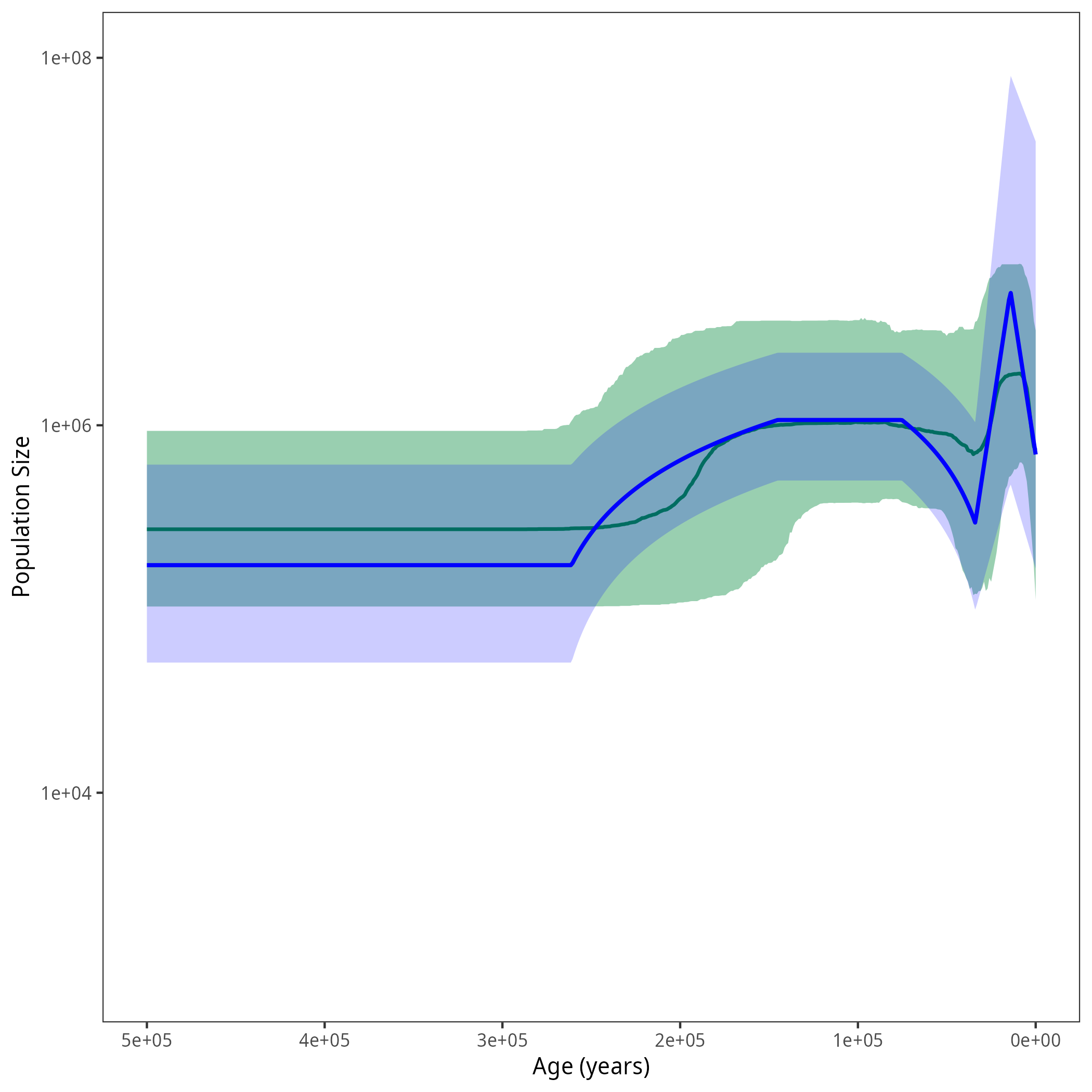
Results
After running your analysis, you can plot the results using the R package RevGadgets and by additionally defining the demographic models from this exercise.
R code
library(RevGadgets)

burnin = 0.1
probs = c(0.025, 0.975)
summary = "median"

num_grid_points = 500
max_age_iso = 5e5
min_age = 0
spacing = "equal"

population_size_log_skyline = "output/horses_iso_skyline_NEs.log"
interval_change_points_log_skyline = "output/horses_iso_skyline_times.log"
df_skyline <- processPopSizes(population_size_log_skyline, interval_change_points_log_skyline, burnin = burnin, probs = probs, summary = summary, num_grid_points = num_grid_points, max_age = max_age_iso, min_age = min_age, spacing = spacing)
p_skyline <- plotPopSizes(df_skyline) + ggplot2::coord_cartesian(ylim = c(1e3, 1e8))

population_size_log = "output/horses_iso_piecewise_6diff_NEs.log"
interval_change_points_log = "output/horses_iso_piecewise_6diff_times.log"
pop_sizes <- readTrace(population_size_log, burnin = burnin)[[1]]
interval_times <- readTrace(interval_change_points_log, burnin = burnin)[[1]]

pop_size_medians = apply(pop_sizes[,grep("size", names(pop_sizes))], 2, median)
pop_size_quantiles = apply(pop_sizes[,grep("size", names(pop_sizes))], 2, quantile, probs = probs)
time_medians =apply(interval_times[,grep("change_points", names(interval_times))], 2, median)

exponential_dem <- function(t, N0, N1, t0, t1){
  alpha = log( N1/N0 ) / (t0 - t1)
  return (N0 * exp( (t0-t) * alpha))
}

linear_dem <- function(t, N0, N1, t0, t1){
  alpha = ( N1-N0 ) / (t1 - t0)
  return (N0 + (t-t0) * alpha)
}

all_combined <- function(t){
  if (t < time_medians[1]){

    return(exponential_dem(t, N0 = pop_size_medians[1], N1 = pop_size_medians[2], t0 = 0, t1 = time_medians[1]))

  } else if (t < time_medians[2]){

    return(exponential_dem(t, N0 = pop_size_medians[2], N1 = pop_size_medians[3], t0 = time_medians[1], t1 = time_medians[2]))

  } else if (t < time_medians[3]){

    return(linear_dem(t, N0 = pop_size_medians[3], N1 = pop_size_medians[4], t0 = time_medians[2], t1 = time_medians[3]))

  } else if (t < time_medians[4]){

    return(pop_size_medians[4])

  } else if (t < time_medians[5]){

    return(linear_dem(t, N0 = pop_size_medians[4], N1 = pop_size_medians[5], t0 = time_medians[4], t1 = time_medians[5]))

  } else {

    return(pop_size_medians[5])

  }
}

all_lower <- function(t){
  if (t < time_medians[1]){

    return(exponential_dem(t, N0 = pop_size_quantiles[1,1], N1 = pop_size_quantiles[1,2], t0 = 0, t1 = time_medians[1]))

  } else if (t < time_medians[2]){

    return(exponential_dem(t, N0 = pop_size_quantiles[1,2], N1 = pop_size_quantiles[1,3], t0 = time_medians[1], t1 = time_medians[2]))

  } else if (t < time_medians[3]){

    return(linear_dem(t, N0 = pop_size_quantiles[1,3], N1 = pop_size_quantiles[1,4], t0 = time_medians[2], t1 = time_medians[3]))

  } else if (t < time_medians[4]){

    return(pop_size_quantiles[1,4])

  } else if (t < time_medians[5]){

    return(linear_dem(t, N0 = pop_size_quantiles[1,4], N1 = pop_size_quantiles[1,5], t0 = time_medians[4], t1 = time_medians[5]))

  } else {

    return(pop_size_quantiles[1,5])

  }
}

all_upper <- function(t){
  if (t < time_medians[1]){

    return(exponential_dem(t, N0 = pop_size_quantiles[2,1], N1 = pop_size_quantiles[2,2], t0 = 0, t1 = time_medians[1]))

  } else if (t < time_medians[2]){

    return(exponential_dem(t, N0 = pop_size_quantiles[2,2], N1 = pop_size_quantiles[2,3], t0 = time_medians[1], t1 = time_medians[2]))

  } else if (t < time_medians[3]){

    return(linear_dem(t, N0 = pop_size_quantiles[2,3], N1 = pop_size_quantiles[2,4], t0 = time_medians[2], t1 = time_medians[3]))

  } else if (t < time_medians[4]){

    return(pop_size_quantiles[2,4])

  } else if (t < time_medians[5]){

    return(linear_dem(t, N0 = pop_size_quantiles[2,4], N1 = pop_size_quantiles[2,5], t0 = time_medians[4], t1 = time_medians[5]))

  } else {

    return(pop_size_quantiles[2,5])

  }
}

grid = seq(0, 3.5e5, length.out = 500)
pop_size_median <- sapply(grid, all_combined)
pop_size_lower <- sapply(grid, all_lower)
pop_size_upper <- sapply(grid, all_upper)

df <-tibble::tibble(.rows = length(grid))
df$value <- pop_size_median
df$lower <- pop_size_lower
df$upper <- pop_size_upper
df$time <- grid

p <- p_skyline +
  ggplot2::geom_line(data = df, ggplot2::aes(x = time, y = value), linewidth = 0.9, color = "blue") +
  ggplot2::geom_ribbon(data = df, ggplot2::aes(x = time, ymin = lower, ymax = upper), fill = "blue", alpha = 0.2)
ggplot2::ggsave("figures/horses_iso_piecewise_6diff.png", p)
Summary
When you are done with all exercises, have a look at the tutorial with heterochronous data or the summary.