Estimating a Time-Calibrated Phylogeny of Fossil and Extant Taxa using Morphological Data

This tutorial comes with a recorded video walkthrough. The video corresponding to each section of the exercise is linked next to the section title. The full playlist is available here:

Overview

This tutorial provides a guide to using RevBayes to perform a simple phylogenetic analysis of extant and fossil bear species (family Ursidae), using morphological data as well as the occurrence times of lineages from the fossil record. A version of this tutorial is published as: Barido-Sottani et al. (2020) “Estimating a time-calibrated phylogeny of fossil and extant taxa using RevBayes”. In Scornavacca, C., Delsuc, F., and Galtier, N., editors, Phylogenetics in the Genomic Era, chapter No. 5.2, pp. 5.2:2–5.2:22. No commercial publisher | Authors open access book.

Introduction

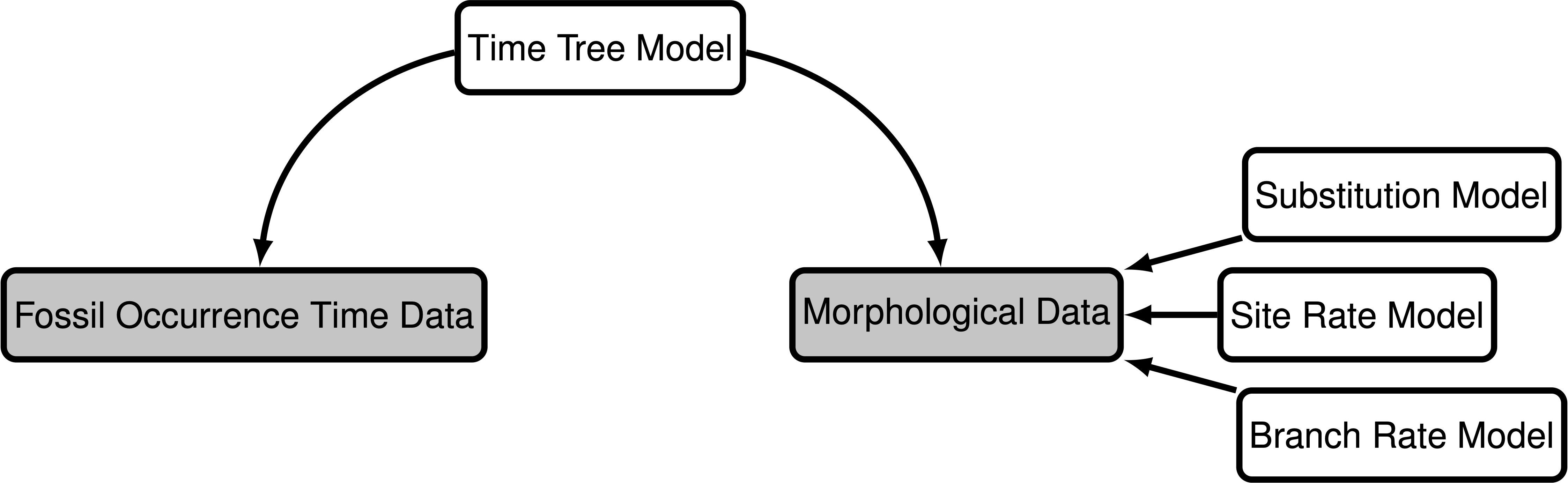
To get an overview of the model, it is useful to think of the model as a generating process for our data. Suppose we would like to simulate our fossil and morphological data; we would consider two components ():

• Time tree model: This is the diversification process that describes how a phylogeny is generated, as well as when fossils are sampled along each lineage on the phylogeny. This component generates the phylogeny, divergence times, and the fossil occurrence data. The tree topology and node ages are parameters of the model that generates our morphological characters.
• Discrete morphological character change model: This model describes how discrete morphological character states change over time on the phylogeny. The generation of observed morphological character states is governed by other model components including the substitution process and variation among characters in our matrix and among branches on the tree.

These two components, or modules, form the backbone of the inference model and reflect our prior beliefs on how the tree, fossil data, and morphological trait data are generated. We will provide a brief overview of the specific models used within each component while pointing to other tutorials that implement alternative models.

Time Tree Model: The Fossilized Birth-Death Process

The fossilized birth death (FBD) process provides a joint distribution on the divergence times of living and extinct species, the tree topology, and the sampling of fossils (Stadler 2010; Heath et al. 2014). The FBD model can be broken into two sub-processes, the birth-death process and the fossilization process.

Birth-Death Process

The birth-death process is a branching process that provides a distribution for the tree topology and divergence times on the tree. We will consider a constant-rate birth-death process (Kendall 1948; Thompson 1975). Specifically, we will assume every lineage has the same constant rate of speciation $\lambda$ and rate of extinction $\mu$ at any moment in time (Nee et al. 1994; Höhna 2015). Speciation and extinction events occur with rate parameters $\lambda$ and $\mu$ respectively, whereby the waiting time between events is exponentially distributed with parameter ($\lambda+\mu$). Then, given an event occurred, the probability of the event being a speciation is ($\lambda$ / ($\lambda+\mu$)) while the probability of the event being an extinction is ($\mu$ / ($\lambda+\mu$)).

The birth-death process depends on two other parameters as well, the origin time and the sampling probability. The origin time, denoted $\phi$, represents the starting time of the stem lineage, which is the age of the entire process. The sampling probability, denoted $\rho$, gives the probability that an extant species is sampled.

The assumption that, at any given time, each lineage has the same speciation rate and extinction rate may not be realistic or valid in some systems. Several models are currently implemented in RevBayes that relax the assumption of constant rates, including:

1. episodic diversification rates (Höhna 2015)
2. environment-dependent diversification rates (Condamine et al. 2018)
3. branch-specific diversification rates (Höhna et al. 2019)
4. diversification rates tied to a species trait (Maddison et al. 2007; Freyman and Höhna 2018; Freyman and Höhna 2019)

Fossilization Process

Given a phylogeny, in this case a phylogeny generated by a birth-death process, the fossilization process provides a distribution for sampling fossilized occurrences of lineages in the tree (Heath et al. 2014). Much like speciation and extinction, fossil sampling is modeled according to a Poisson process with rate parameter $\psi$. This means that each lineage has the same constant rate of producing a fossil. As a result, along a given lineage, the time between fossilization events is exponentially distributed with rate $\psi$.

One key assumption of the FBD model is that each fossil represents a distinct fossil specimen. However, if certain taxa persist through time and fossilize particularly well, then the same taxon may be sampled at different stratigraphic ages. These fossil data are commonly represented by only the first and last appearances of a fossil morphospecies. In this case one might want to consider the fossilized birth-death range process (Stadler et al. 2018) in RevBayes to model the stratigraphic ranges of fossil occurrences.

Accounting for Fossil Age Uncertainty

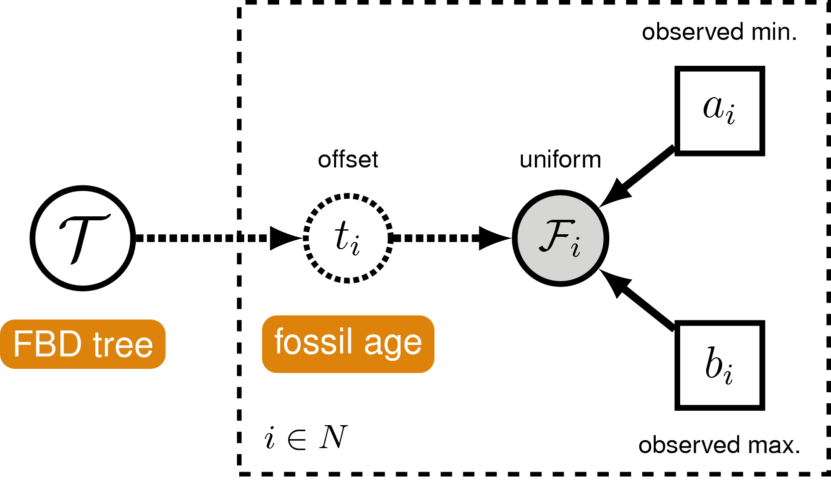
Often, there is uncertainty around the age of each fossil, which is typically represented as an interval of the minimum and maximum possible ages. Moreover, a recent study demonstrated using simulated data that ignoring uncertainty in fossil occurrence dates can lead to biased estimates of divergence times (Barido-Sottani et al. 2019). RevBayes allows fossil occurrence time uncertainty to be modeled by directly treating it as part of the likelihood of the fossil data given the time tree. We model this by assuming the likelihood of a particular fossil occurrence $\mathcal{F}_i$ is zero if the inferred age $t_i$ occurs outside the time interval $(a_i,b_i)$ and some non-zero likelihood when the fossil is placed within the interval. Specifically, we will assume the fossil could occur anywhere within the observed interval with uniform probability, this means that the likelihood is equal to one if the inferred fossil age is consistent with the observed fossil interval:

The incorporation of uncertainty around the fossil occurrence data is shown graphically as a part of our model in .

Modeling Discrete Morphological Character Change

Given a phylogeny, the discrete morphological character change model will describe how traits change along each lineage, resulting in the observed character states of fossils and living species. In our case, the phylogeny and fossil occurrences are generated from the FBD process and we will be modeling the evolution of discrete morphological characters with two states. There are three main components to consider with modeling discrete morphological traits (as shown in ): the substitution model, the branch rate model, and the site rate model.

Substitution Model

The substitution model describes how discrete morphological characters evolve over time. We will be using the Mk model (Lewis 2001), a generalization of the Jukes-Cantor (Jukes and Cantor 1969) model described for nucleotide substitutions. The Mk model assumes that all transitions from one state to another occur at the same rate, for all $k$ states. Since the characters used in this tutorial all have two states, we will specifically be using a model where $k=2$. Thus, a transition from state 0 to state 1 is equally as likely as a transition from state 1 to state 0. For this tutorial, we focus on binary (2-state) characters for simplicity, but it is important to note that RevBayes can also accommodate multistate characters as well.

The evolution of discrete morphological characters is thought to occur at a very slow rate. Moreover, once some characters transition to a certain state, they rarely transition back, which means that the assumption of symmetric rates is likely violated my many empirical datasets (Wright et al. 2016; Wright 2019). We can accommodate asymmetric transition rates for each state using alternative models in RevBayes. Additionally, if some characters change symmetrically while others change asymmetrically, it is possible to partition the character matrix to account for model heterogeneity in the matrix.

Branch-Rate Model

The branch-rate model describes how rates of morphological state transitions vary among branches in the tree. Each lineage in the phylogeny is assigned a value that acts as a scalar for the rate of character evolution. In our case we assume each branch has the same rate of evolution, this is a strict morphological clock (Zuckerkandl and Pauling 1962), which is analogous to a strict molecular clock. It is also possible to account for variation in rates among branches. These “relaxed-clock” models are commonly applied to molecular datasets and are currently implemented in RevBayes (see the Clocks and Time Trees tutorial).

Site-Rate Model

The rate of character evolution can often vary from site to site, i.e. from one column in the matrix to another. Under the site-rate model, a scalar is applied to each character to account for variation in relative rates. In our case we will assume that each character belongs to one of four rate categories from the discretized gamma distribution (Yang 1994), which is parameterized by shape parameter $\alpha$ and number of rate categories $n$. Normally a gamma distribution requires shape $\alpha$ and rate $\beta$ parameters, however, we set our site rates to have a mean of one, which results in the constraint $\alpha=\beta$, thus eliminating the second parameter. The parameter $n$ breaks the gamma distribution into $n$ equiprobable bins where the rate value of each bin is equal to its mean or median.

Putting Together the Complete Phylogenetic Model

We have outlined the specific components forming the processes that govern the generation of the time tree and morphological character data; and together these modules make up the complete phylogenetic model. shows the complete probabilistic graphical model that includes all of the parameters we will use in this tutorial (see Höhna et al. (2014) for more on graphical models for statistical phylogenetics).

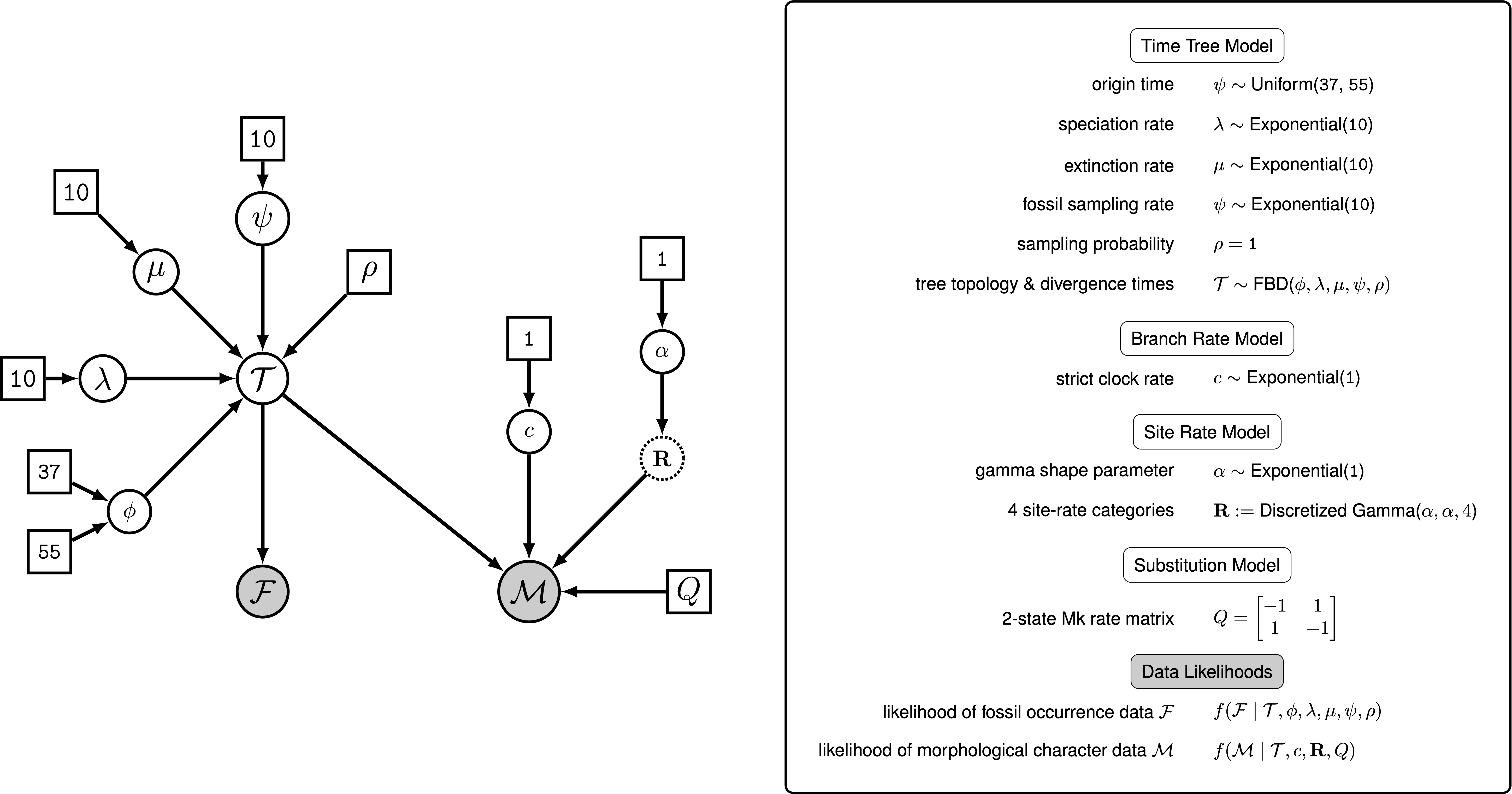
The parameters represented as stochastic nodes (solid white circles) in are unknown random variables that are estimated in our analysis. For each of these parameters, we assume a prior distribution that describes our uncertainty in that parameter’s value. For example, we apply an exponential distribution with a rate of 10 as a prior on the mutation rate: $\mu\sim$ Exponential(10). The parameters represented as constant nodes (white boxes) are fixed to “known” or asserted values in the analysis.

Alternative Models and Analyses

The model choices and analysis in this tutorial focus on a simple example. Importantly, the modular design of RevBayes allows for many model choices to be swapped with more complex or biologically relevant processes for a given system. Analyses of a wide range of data types are also implemented in RevBayes (e.g. nucleotide sequences, historical biogeographic ranges). Moreover, it is possible to fully integrate models describing the generation of data from different sources like in the “combined-evidence” approach (Ronquist et al. 2012; Zhang et al. 2016; Gavryushkina et al. 2017) in a single, hierarchical Bayesian model. Some researchers may wish to perform analyses with node calibrations Ultimately, for any statistical analysis of empirical data, it is important to consider the processes governing the generation of those data and how they can be represented in a hierarchical model.

Exercise: Phylogenetic Inference under the Fossilized Birth-Death Process

In this exercise, we will create a script in Rev, the interpreted programming language used by RevBayes, that defines the model outlined above and specifies the details of the MCMC simulation. This script can be executed in RevBayes to complete the full analysis. We conclude the exercise by evaluating the performance of the MCMC and summarizing the results.

Data and Files

On your own computer or your remote machine, create a directory called RB_FBD_Tutorial (or any name you like).

Then, navigate to the folder you created and make a new one called data.

In the data folder, add the following files (click on the hyperlinked file names to download):

• bears_taxa.tsv: a tab-separated table listing the 18 bear species in our analysis (both fossil and extant) and their occurrence age ranges (minimum and maximum ages). For extant taxa, the minimum age is 0.0 (i.e. the present).
• bears_morphology.nex: a matrix of 62 discrete, binary (coded 0 or 1) morphological characters for our 18 species of fossil and extant bears.

Now you can create a separate file for the Rev script.

In the RB_FBD_Tutorial directory created above, create a blank file called FBD_tutorial.Rev and open it in a text editor.

It is also possible to execute this entire tutorial in the RevBayes console.

The file FBD_tutorial.Rev will contain all of the instructions required to load the data, assemble the different model components used in the analysis, and configure and run the Markov chain Monte Carlo (MCMC) analysis. Once you finish writing this file, you can compare your script with the example provide with this tutorial (see links above).

Importing Data into RevBayes

We will begin our Rev script by loading in the two data files that were downloaded and saved to the data directory. In RevBayes, we use functions to read the contents of files and assign them to variables in our workspace. First, we will create a variable called taxa that will contain the data from bears_taxa.tsv.

taxa <- readTaxonData("data/bears_taxa.tsv")

The file bears_taxa.tsv contains a table with all of the fossil and extant bear species names in the first column, their minimum age in the second column and their maximum age in the third column. We use the function readTaxonData to load this table into the workspace.

Next, we will import the morphological character matrix from bears_morphology.nex and assign it to the variable morpho. In this exercise, we are using a NEXUS-formatted data file, but it is worth noting that several other file-types are acceptable depending on the kind of data (e.g., FASTA for molecular data).

morpho <- readDiscreteCharacterData("data/bears_morphology.nex")

Here, we use the function readDiscreteCharacterData to load a data matrix to the workspace from a formatted file. This function can be used for discrete morphological data as well as molecular sequence data (e.g., nucleotides, amino acids).

Helper Variables

Before we begin specifying the hierarchical model, it is useful to instantiate some “helper variables” that will be used in our model and MCMC specification throughout our script.

First, we will create a new constant node called n_taxa that is equal to the number of species in our analysis (18).

n_taxa <- taxa.size()

Next, we will create a workspace variable called moves, which is a vector that will contain all of the MCMC moves used to propose new states for every stochastic node in the model graph. Each time a new stochastic node is created in the model, we can append the corresponding moves to this vector.

moves = VectorMoves()

One important distinction here is that moves is part of the RevBayes workspace and not the hierarchical model. Thus, we use the workspace assignment operator = instead of the constant node assignment <-.

The Fossilized Birth-Death Process

Speciation and Extinction Rates

Two key parameters of the FBD process are the speciation rate (the rate at which lineages are added to the tree, denoted by $\lambda$ in ) and the extinction rate (the rate at which lineages are removed from the tree, $\mu$ in ). We will place exponential priors on both of these values, meaning we assume each parameter is drawn independently from a different exponential distribution, where each distribution has a rate parameter equal to 10. Note that an exponential distribution with a rate of 10 has an expected value (mean) of 1/10.

Create the exponentially distributed stochastic nodes for the speciation_rate and extinction_rate using the ~ stochastic assignment operator.

speciation_rate ~ dnExponential(10)
extinction_rate ~ dnExponential(10)

The ~ operator in Rev instantiates a stochastic node in the model (i.e., a solid circle in ). Every stochastic node must be defined by a distribution. In this case, we use the Exponential. In the Rev language, every distribution has the prefix dn to make it easier to locate the various distributions in the Rev language documentation (https://revbayes.com/documentation). When a stochastic node is created in the model, the distribution function assigns it an initial value by drawing a random value from the prior distribution and assigns the node to the named variable.

For every stochastic node we declare, we must also specify proposal algorithms (called moves) to sample the value of the parameter in proportion to its posterior probability. If a move is not specified for a stochastic node, then it will not be estimated, but fixed to its initial value.

The extinction rate and speciation rate are both positive, real numbers (i.e., non-negative floating point variables). For both of these nodes, we will use a scaling move (mvScale), which proposes multiplicative changes to a parameter.

moves.append( mvScale(speciation_rate, weight=1) )

moves.append( mvScale(extinction_rate, weight=1) )

You will also notice that each move has a specified weight. This option indicates the frequency a given move will be performed in each MCMC cycle. In RevBayes, the MCMC is executed by default with a schedule of moves at each step of the chain, instead of just one move per step, as is done in MrBayes (Ronquist and Huelsenbeck 2003) or BEAST (Drummond et al. 2012; Bouckaert et al. 2014). Here, if we were to run our MCMC with our current vector of 2 moves each with a weight of 1, then our move schedule would perform 2 moves in each cycle. Within a cycle, an individual move is chosen from the move list in proportion to its weight. Therefore, with both moves assigned weight=1, each has an equal probability of being executed and will be performed on average one time per MCMC cycle. For more information on moves and how they are performed in RevBayes, please refer to the Introduction to Markov chain Monte Carlo (MCMC) Sampling and Nucleotide substitution models tutorials.

In addition to the speciation ($\lambda$) and extinction ($\mu$) rates, we may also be interested in inferring the net diversification rate ($\lambda - \mu$) and the turnover ($\mu/\lambda$). Since these parameters can each be expressed as a deterministic transformation of the speciation and extinction rates, we can monitor their values (i.e., track their values and print them to a file) by creating two deterministic nodes using the := deterministic assignment operator.

diversification := speciation_rate - extinction_rate
turnover := extinction_rate/speciation_rate

Deterministic nodes are represented by circles with dotted borders in a probabilistic graphical model. To maintain the simplicity of the model in , the diversification rate and turnover are not shown.

Extant Sampling Probability

Every extant bear species is represented in this dataset. Therefore, we will fix the probability of sampling an extant lineage ($\rho$ in ) to 1. The parameter rho will be specified as a constant node (new values for rho will not be sampled in the MCMC) using the <- constant assignment operator.

rho <- 1.0

Because $\rho$ is a constant node, we do not have to assign a move to this parameter because we assume the value is known and fixed.

Fossil Sampling Rate

Since our data set includes serially sampled lineages, we must also account for the rate of sampling through time. This is the fossil sampling (or recovery) rate ($\psi$ in ), which we will instantiate as a stochastic node named psi. As with the speciation and extinction rates (see ), we will use an exponential prior on this parameter and apply a scale move to sample values from the posterior distribution.

psi ~ dnExponential(10) 

moves.append( mvScale(psi, weight=1) )

Origin Time

The FBD process is conditioned on the origin time ($\phi$ in ), which requires specification of a node representing the age of the clade. We will set a uniform distribution on the origin age, with the lower bound set at the age of the oldest bear fossil (37 My) and the higher bound of 55 My set to the age of the most recent common ancestor of crown Carnivora estimated by recent studies (dos Reis et al. 2012). For the move, we will use a sliding window move (mvSlide), which samples a parameter uniformly within an interval (defined by the half-width delta, which is set to 1 by default). Sliding window moves can be problematic for small values, as the window may overlap zero. However, our prior on the origin age excludes values $\leq 37.0$, so this is not an issue.

origin_time ~ dnUnif(37.0, 55.0)

moves.append( mvSlide(origin_time, weight=1.0) )

The FBD Tree

Now that we have specified all of the parameters of the FBD process ($\lambda$, $\mu$, $\phi$, $\psi$), we will use these parameters to instantiate the stochastic node representing the time-calibrated tree that we will call fbd_tree. The fbd_tree ($\mathcal{T}$ in ) is generated by a fossilized birth-death distribution and is conditionally dependent on $\lambda$, $\mu$, $\phi$, and $\psi$. The FBD distribution function fnFBDP takes the FBD parameters as arguments as well as the taxa variable which specifies the number of terminal taxa as well as the taxon labels.

fbd_tree ~ dnFBDP(origin=origin_time, lambda=speciation_rate, mu=extinction_rate, psi=psi, rho=rho, taxa=taxa)

Next, in order to sample from the posterior distribution of trees, we need to specify moves that propose changes to the topology (e.g. mvFNPR) and node times (e.g. mvNodeTimeSlideUniform). We also include a proposal that will collapse or expand a fossil branch (mvCollapseExpandFossilBranch), thus sampling trees where a given fossil is either a sampled ancestor or a sampled tip. In addition, when conditioning on the origin time, we also need to explicitly sample the root age (mvRootTimeSlideUniform).

moves.append( mvFNPR(fbd_tree, weight=15.0) )
moves.append( mvCollapseExpandFossilBranch(fbd_tree, origin_time, weight=6.0) )

moves.append( mvNodeTimeSlideUniform(fbd_tree, weight=40.0) )
moves.append( mvRootTimeSlideUniform(fbd_tree, origin_time, weight=5.0) )

Note that we specified a higher move weight for each of the proposals operating on fbd_tree than we did for the previous stochastic nodes. This means that our move schedule will propose fifteen times as many new topologies via the mvFNPR move as it will new values of speciation_rate using mvScale, for example. By increasing the number of times new values are proposed for a parameter, we are increasing the sampling intensity for that parameter. Typically, we do this for parameters that we are particularly interested in or for parameters that tend to induce long mixing times. A node like $\mathcal{T}$ in our graphical model () represents a complex set of variables: the tree topology and all divergence times. Moreover, the likelihoods of our fossil occurrence data and the morphological character data are both conditionally dependent on the time tree. Such complex variables require more extensive sampling than other nodes.

Sampling Fossil Occurrence Times

We need to account for uncertainty in the age estimates of our fossils using the observed minimum and maximum stratigraphic ages that are provided in the file bears_taxa.tsv. We can represent the fossil likelihood using any uniform distribution that is non-zero when the likelihood is equal to one (see ). For example, if $t_i$ is the inferred fossil age and $(a_i,b_i)$ is the observed stratigraphic interval, we know the likelihood is equal to one when $a_i < t_i < b_i$, or equivalently $t_i - b_i < 0 < t_i - a_i$. So we can represent this likelihood using a uniform random variable, uniformly distributed in $(t_i - b_i, t_i - a_i)$ and clamped at zero.

To do this, we will get all the fossils from the tree and use a for loop to iterate over them. For each fossil observation, we will create a uniform random variable representing the likelihood, based on the minimum and maximum ages specified in the file bears_taxa.tsv.

fossils = fbd_tree.getFossils()
for(i in 1:fossils.size())
{
    t[i] := tmrca(fbd_tree, clade(fossils[i]))

    a_i = fossils[i].getMinAge()
    b_i = fossils[i].getMaxAge()

    F[i] ~ dnUniform(t[i] - b_i, t[i] - a_i)
    F[i].clamp( 0 )
}

Finally, we will add a move that samples the ages of all the fossils on the tree.

moves.append( mvFossilTimeSlideUniform(fbd_tree, origin_time, weight=5.0) )

Monitoring Parameters of Interest

There are additional parameters that may be of particular interest to us that are not directly sampled as part of the graphical model defined thus far. As with the diversification and turnover nodes specified in , we can create deterministic nodes to sample the posterior distributions of these parameters. Here we will create a deterministic node called num_samp_anc that will compute the number of sampled ancestors in our fbd_tree.

num_samp_anc := fbd_tree.numSampledAncestors();

We are also interested in the age of the most-recent-common ancestor (MRCA) of all living bears. To monitor this age in our MCMC sample, we must use the clade function to identify the node corresponding to the MRCA. Once this clade is defined we can instantiate a deterministic node called age_extant that will record the age of the MRCA of all living bears, using the tmrca() function.

clade_extant = clade("Ailuropoda_melanoleuca","Tremarctos_ornatus","Melursus_ursinus",
                    "Ursus_arctos","Ursus_maritimus","Helarctos_malayanus",
                    "Ursus_americanus","Ursus_thibetanus")
age_extant := tmrca(fbd_tree, clade_extant)

In the same way we monitored the MRCA of the extant bears, we can also monitor the age of a fossil taxon that we may be interested in recording. We will monitor the marginal distribution of the age of Kretzoiarctos beatrix, which is sampled between 11.2–11.8 My.

age_Kretzoiarctos_beatrix := tmrca(fbd_tree, clade("Kretzoiarctos_beatrix"))

Modeling the Evolution of Binary Morphological Characters

The next part of the graphical model we will define specifies the model of morphological character evolution. This component includes the substitution model, the model of rate variation among characters, and the model of rate variation among branches ().

As stated in the section, we will use the Mk model to model our data. Because the Mk model is a generalization of the Jukes-Cantor model (Jukes and Cantor 1969), we will initialize our instantaneous rate matrix from a Jukes-Cantor matrix. The constant node Q_morpho corresponds to the two-state rate matrix $Q$ in .

Q_morpho <- fnJC(2)

We will assume that rates vary among characters in our data matrix according to a discretized gamma distribution (described in the section on ). For this model, we create a vector of rates named rates_morpho which is the product of a function fnDiscretizeGamma() that divides up a gamma distribution into a set of equal-probability bins ($\mathbf{R}$ in Figure ). Here, our only stochastic node is alpha_morpho ($\alpha$ in (missing reference), which is the shape parameter of the discretized gamma distribution.

alpha_morpho ~ dnExponential( 1.0 )
rates_morpho := fnDiscretizeGamma( alpha_morpho, alpha_morpho, 4 )

moves.append( mvScale(alpha_morpho, weight=5.0) )

The phylogenetic model also assumes that each branch has a rate of morphological character change. For simplicity, we will assume a strict morphological clock — meaning that every branch has the same rate rate represented by the stochastic node clock_morpho ($c$ in ), which is drawn from an exponential distribution (see the section).

clock_morpho ~ dnExponential(1.0)

moves.append( mvScale(clock_morpho, weight=4.0) )

The Phylogenetic CTMC

If you refer to , you will see that we have defined almost all of the components of the complete model except for the observed node representing our morphological character data ($\mathcal{M}$). The character matrix is a clamped stochastic node that is generated by a phylogenetic continuous-time Markov chain (CTMC) distribution. This node is conditionally dependent on the time tree ($\mathcal{T}$: fbd_tree), clock rate ($c$: clock_morpho), site rates ($\mathbf{R}$: rates_morpho), and the two-state Mk rate matrix ($Q$: Q_morpho). With all of these nodes instantiated in the graphical model, we can now connect the components by defining the node representing our observed morphological data.

There are some unique aspects to specifying a phylogenetic CTMC for morphological data. You will notice that we have an option called coding. This option allows us to condition on biases in the way the morphological data were collected (i.e., ascertainment bias). By setting coding=variable we can correct for coding only variable characters (discussed in (Lewis 2001)).

phyMorpho ~ dnPhyloCTMC(tree=fbd_tree, siteRates=rates_morpho, branchRates=clock_morpho, Q=Q_morpho, type="Standard", coding="variable")
phyMorpho.clamp(morpho)

Now that we have defined our complete model, we can create a workspace variable that packages the entire model graph. This makes it easy to pass the whole model to functions that will set up our MCMC analysis. This variable is created using the model() function, which takes only a single node in the graph. We will use the fbd_tree node, but you can try this with an alternative node (e.g., clock_morpho, rho, etc.). As long as you have established all of the connections among the model parameters, the model() function will find every other node by traversing the edges of the graph ().

mymodel = model(fbd_tree)

Monitoring Variables

We have defined the full probabilistic graphical model shown in and we are now ready to specify the details of our MCMC analysis. The first step in setting up the analysis is to create monitors that will record the values of each parameter in our model for every sampled cycle of the MCMC. The sampled values are saved to file (or printed to screen) and can be summarized when our MCMC simulation is complete.

Let’s create three different monitor objects for this analysis. To manage the monitors in RevBayes, we create another workspace variable called monitors that is a vector containing the three monitor variables.

monitors = VectorMonitors()

We will append our first monitor to the monitors vector. This will create a file called bears.log in a directory called output (if this directory does not already exist, RevBayes will create it). The function mnModel() initializes a monitor that saves all of the numerical parameters in the model to a tab-delineated file. This file is useful for summarizing marginal posteriors in statistical plotting tools like Tracer (Rambaut et al. 2018) or R (R Core Team 2020). We will exclude the F vector from logging, as it is purely used as an auxiliary variable for estimating fossil ages, and is clamped to 0. Additionally, we also specify how frequently we sample our Markov chain by setting the printgen option. We will sample every 10 cycles of our MCMC. Importantly, we also specify how frequently we sample our Markov chain by setting the printgen option. We will sample every 10 cycles of our MCMC.

monitors.append( mnModel(filename="output/bears.log", printgen=10, exclude = ["F"]) )

You may think that sampling every 10 generations may be too frequent to avoid correlation between samples in our MCMC. However, recall that a single “generation” in RevBayes performs a schedule of moves that is determined by the number of moves in the moves vector and the weights assigned to those moves (see the section). Thus, a single generation in this analysis will involve 26 moves, so if we record every 10 generations, there will be 260 moves between each sample.

We want to create a separate file containing samples of the tree and branch lengths since these will not be saved by the monitor defined above. To save the tree parameter, we can use the mnFile() function that saves specific parameters to a file. We indicate the parameters by including them in the function’s options.

monitors.append( mnFile(filename="output/bears.trees", printgen=10, fbd_tree) )

The final monitor will print updates of our MCMC to the screen. The screen monitor function, mnScreen() allows us to add parameters in our model that will be displayed along with a few default values (including the current iteration, posterior, likelihood, and prior). We will monitor the age of the MRCA of the living bears, the number of sampled ancestors, and the origin time.

monitors.append( mnScreen(printgen=10, age_extant, num_samp_anc, origin_time) )

Setting up and Running the MCMC Sampler

Our Rev script specifies the three major parts of our MCMC analysis: a model (mymodel), a list of MCMC proposals (moves), and a way to save the values sampled by our Markov chain (monitors). With these three components, we can set up our analysis using the mcmc() function. This function creates a workspace variable that we can use to execute the MCMC simulation.

mymcmc = mcmc(mymodel, monitors, moves)

Using our variable mymcmc, we can execute the run() member method to start our MCMC sampler.

mymcmc.run(generations=10000)

Finally, since we are going to save this analysis in a script file and run it in RevBayes, it is useful to include a statement that will quit the program when the run is complete.

q()

Your script is now complete!

Save the FBD_tutorial.Rev file in the RB_FBD_Tutorial directory.

Execute the Analysis Script in RevBayes

With your script complete and data files in the proper locations, you can execute the FBD_tutorial.Rev script in RevBayes.

Run the RevByes executable.

On Unix systems, if the RevBayes is in your path, you simply need to navigate to the RB_FBD_Tutorial directory and type rb.

If the RevBayes executable is not in your path, you can execute it and then change your working directory using the setwd() function which takes the absolute path to your directory as an argument.

setwd("<path to>/RB_FBD_Tutorial")

Once RevBayes is in the correct directory (RB_FBD_Tutorial), you can then use the source() function to feed RevBayes your master script file (FBD_tutorial.Rev).

source("FBD_tutorial.Rev")

   Processing file "FBD_tutorial.Rev"
   Successfully read one character matrix from file 'data/bears_morphology.nex'

   Running MCMC simulation
   This simulation runs 1 independent replicate.
   The simulator uses 11 different moves in a random move schedule with 26 moves per iteration
   ...

This will execute the analysis and you should see the various parameters—specified when you initialized the screen monitor—printed to the screen every 10 generations. When the analysis is complete, RevBayes will quit and you will have a new directory called output that will contain all of the files you specified with the monitors.

Results

Two files are created by the monitors in the section. These files, located in the output directory contain the record of values sampled for the various parameters of the model over the course of the MCMC. In the following sections, we will assess the performance of our MCMC sampler and summarize the marginal posterior distributions of numerical parameters (in the file bears.log) and the time-calibrated phylogeny (in the file bears.trees).

Evaluating the MCMC Sampler

The first step when analyzing the output of an MCMC run is to check whether the chain has converged on the stationary distribution and sampled effectively (i.e., achieved “good mixing”). This can be done by loading the parameter log, in our case the file bears.log, in a program such as Tracer (Rambaut et al. 2018), shown in .

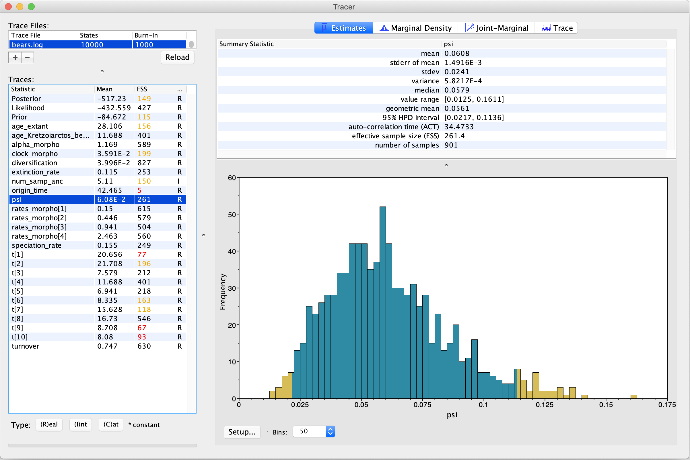
On the left side is a panel summarizing all the parameters appearing in the log, with their mean estimate and ESS value (effective sample size). The ESS of a parameter determines whether the chain has adequately sampled the associated variable: values above 200 are considered “good”, whereas values below 200, highlighted by Tracer in yellow or red, indicate poor mixing. Explicitly, the ESS measures the degree of independence between samples and parameters with signatures of autocorrelation between samples are indicative of an inadequate sampler.

Here we can see that the chain has mixed well for some parameters, but not others. In particular, we see low ESS values for the origin time (origin_time) and the ages of some fossil tips (t[1], t[9], and t[10]). This may indicate that the MCMC sampler has not converged on the stationary distribution for these parameters, which are associated with the FBD tree. What this assessment reveals is that we did not perform enough proposals for these parameters. Thus, it will be important to run the MCMC for more generations (specified in the section) and/or increase the weights of moves applied to these stochastic nodes (e.g., the mvSlide applied to origin_time in the section). For more details on diagnosing convergence of MCMC samples under the FBD model, please see the tutorial on combined-evidence analysis in RevBayes.

Summarizing the Tree

Once we are certain that our MCMC has effectively sampled the joint posterior distribution of our model parameters, we can summarize the tree topology, branch times, and fossil ages that were saved to output/bears.trees using some built-in RevBayes functions.

Run the RevByes executable, making sure that the working directory is RB_FBD_Tutorial.

The file bears.trees contains the trees and associated parameters that were sampled every 10 generations by our monitor. In RevBayes, we often refer to a set of samples from our MCMC as a “trace”.

Begin by loading the tree trace into RevBayes from the bears.trees file.

trace = readTreeTrace("output/bears.trees")

   Processing file "<path to>/RB_FBD_Tutorial/output/bears.trees"

Progress:
0---------------25---------------50---------------75--------------100
********************************************************************

By default, a burn-in of 25% is used when reading in the tree trace (250 trees in our case). Note that this is different from Tracer, which uses a burn-in fraction of 10% by default. You can specify a different burn-in fraction, say 50%, by typing the command trace.setBurnin(500).

Now we will use the mccTree() function to return a maximum clade credibility (MCC) tree. The MCC tree is the tree with the maximum product of the posterior clade probabilities. When considering trees with sampled ancestors, we refer to the maximum sampled ancestor clade credibility (MSACC) tree (Gavryushkina et al. 2017).

mccTree(trace, file="output/bears.mcc.tre" )

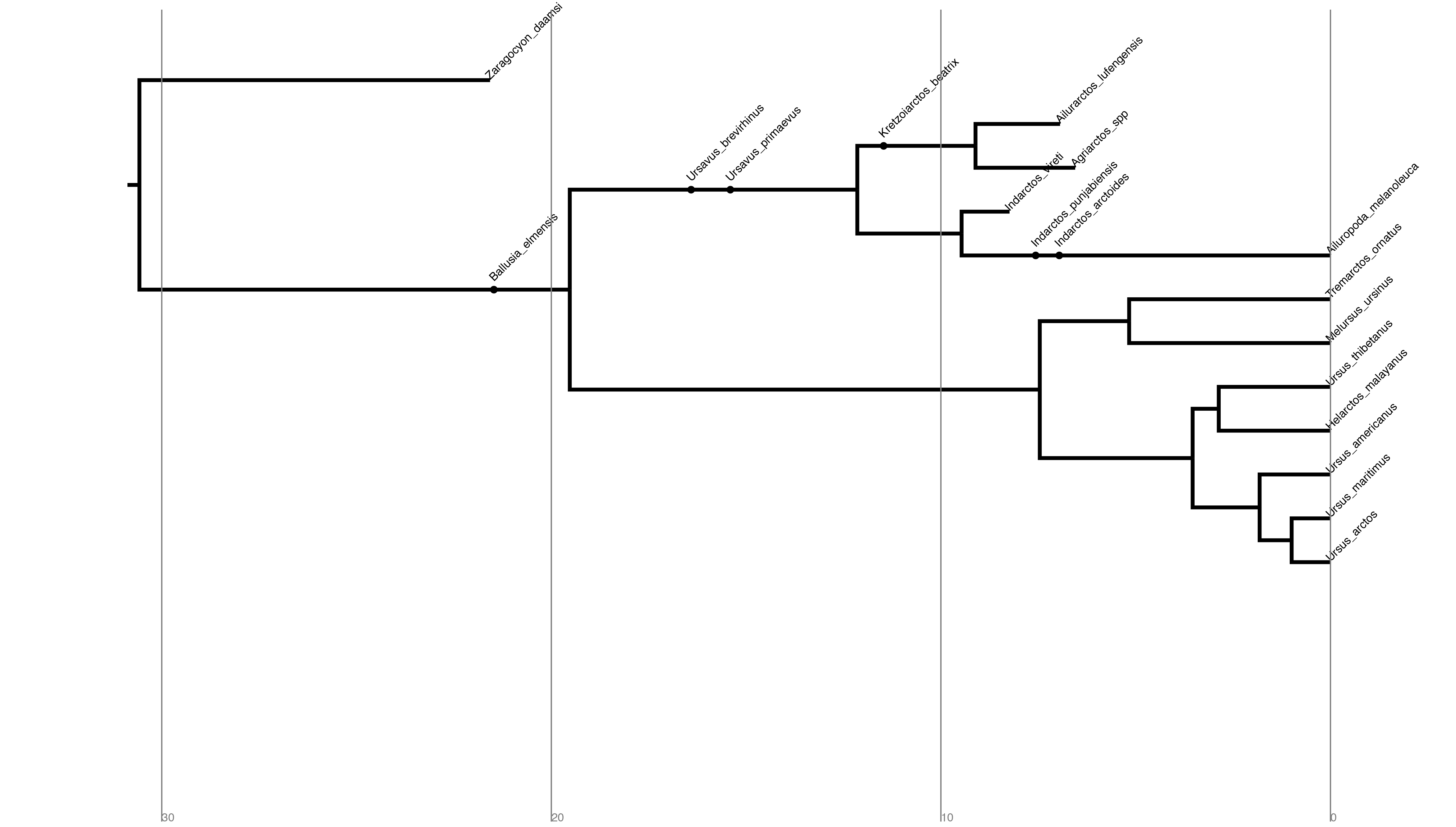
When there are sampled ancestors present, visualizing the tree can be fairly difficult in traditional tree viewers. When there are sampled ancestors present, visualizing the tree can be fairly difficult in traditional tree viewers. We will make use of a browser-based tree visualization tool called IcyTree (Vaughan 2017), which can be accessed at https://icytree.org. IcyTree has many unique options for visualizing phylogenetic trees and can produce publication-quality vector image files (i.e. SVG). Additionally, it correctly represents sampled ancestors on the tree as nodes, each with only one descendant ().

Navigate to https://icytree.org and open the file output/bears.mcc.tre in IcyTree.

Try to replicate the tree in (Hint: Style > Mark Singletons)

⇨ Why might a node with a sampled ancestor be referred to as a singleton?

⇨ How can you see the names of the fossils that are putative sampled ancestors?

⇨ What is the posterior probability that Zaragocyon daamsi is a sampled ancestor?

Summary

In this tutorial, we have introduced core information about how morphological and age information are modeled for use with the FBD model in RevBayes. We have also discussed important aspects of executing and summarizing MCMC analysis. This exercise uses a simplified data set and set of models for analysis of fossil and extant data. Most researchers working on living taxa have access to molecular (including genomic) data and may be interested in applying these methods to much larger datasets and more complex problems. Note that the goal of this tutorial is to provide a concise introduction to the framework for analysis of paleontological and neontological data in RevBayes. For more information on how to apply RevBayes datasets combining morphological and molecular characters, please refer to the following tutorials:

1. Combined-Evidence Analysis and the Fossilized Birth-Death Process for Analysis of Extant Taxa and Fossil Specimens
2. Combined-Evidence Analysis and the Fossilized Birth-Death Process for Stratigraphic Range Data

1. Barido-Sottani J., Aguirre-Fernández G., Hopkins M.J., Stadler T., Warnock R. 2019. Ignoring stratigraphic age uncertainty leads to erroneous estimates of species divergence times under the fossilized birth–death process. Proceedings of the Royal Society B: Biological Sciences. 286:20190685.
2. Bouckaert R., Heled J., Kühnert D., Vaughan T., Wu C.-H., Xie D., Suchard M.A., Rambaut A., Drummond A.J. 2014. BEAST 2: a software platform for Bayesian evolutionary analysis. PLoS Computational Biology. 10:e1003537. 10.1371/journal.pcbi.1003537
3. Condamine F.L., Rolland J., Höhna S., Sperling F.A.H., Sanmartín I. 2018. Testing the role of the Red Queen and Court Jester as drivers of the macroevolution of Apollo butterflies. Systematic Biology. 67:940–964.
4. Drummond A.J., Suchard M.A., Xie D., Rambaut A. 2012. Bayesian phylogenetics with BEAUti and the BEAST 1.7. Molecular Biology and Evolution. 29:1969–1973. 10.1093/molbev/mss075
5. Freyman W.A., Höhna S. 2019. Stochastic character mapping of state-dependent diversification reveals the tempo of evolutionary decline in self-compatible Onagraceae lineages. Systematic Biology. 68:505–519.
6. Freyman W.A., Höhna S. 2018. Cladogenetic and anagenetic models of chromosome number evolution: a Bayesian model averaging approach. Systematic Biology. 67:1995–215.
7. Gavryushkina A., Heath T.A., Ksepka D.T., Stadler T., Welch D., Drummond A.J. 2017. Bayesian Total-Evidence Dating Reveals the Recent Crown Radiation of Penguins. Systematic Biology. 66:57–73. 10.1093/sysbio/syw060
8. Heath T.A., Huelsenbeck J.P., Stadler T. 2014. The fossilized birth-death process for coherent calibration of divergence-time estimates. Proceedings of the National Academy of Sciences. 111:E2957–E2966. 10.1073/pnas.1319091111
9. Höhna S. 2015. The time-dependent reconstructed evolutionary process with a key-role for mass-extinction events. Journal of Theoretical Biology. 380:321–331. http://dx.doi.org/10.1016/j.jtbi.2015.06.005
10. Höhna S., Freyman W.A., Nolen Z., Huelsenbeck J.P., May M.R., Moore B.R. 2019. A Bayesian Approach for Estimating Branch-Specific Speciation and Extinction Rates. bioRxiv. 10.1101/555805
11. Höhna S., Heath T.A., Boussau B., Landis M.J., Ronquist F., Huelsenbeck J.P. 2014. Probabilistic Graphical Model Representation in Phylogenetics. Systematic Biology. 63:753–771. 10.1093/sysbio/syu039
12. Jukes T.H., Cantor C.R. 1969. Evolution of Protein Molecules. Mammalian Protein Metabolism. 3:21–132. 10.1016/B978-1-4832-3211-9.50009-7
13. Kendall D.G. 1948. On the Generalized "Birth-and-Death" Process. The Annals of Mathematical Statistics. 19:1–15. 10.1214/aoms/1177730285
14. Lewis P.O. 2001. A Likelihood Approach to Estimating Phylogeny from Discrete Morphological Character Data. Systematic Biology. 50:913–925. 10.1080/106351501753462876
15. Maddison W.P., Midford P.E., Otto S.P. 2007. Estimating a binary character’s effect on speciation and extinction. Systematic Biology. 56:701. 10.1080/10635150701607033
16. Nee S., May R.M., Harvey P.H. 1994. The Reconstructed Evolutionary Process. Philosophical Transactions: Biological Sciences. 344:305–311. 10.1098/rstb.1994.0068
17. Rambaut A., Drummond A.J., Xie D., Baele G., Suchard M.A. 2018. Posterior Summarization in Bayesian Phylogenetics Using Tracer 1.7. Systematic Biology. 67:901–904. 10.1093/sysbio/syy032
18. Ronquist F., Huelsenbeck J.P. 2003. MrBayes 3: Bayesian phylogenetic inference under mixed models. Bioinformatics. 19:1572–1574. 10.1093/bioinformatics/btg180
19. Ronquist F., Klopfstein S., Vilhelmsen L., Schulmeister S., Murray D.L., Rasnitsyn A.P. 2012. A total-evidence approach to dating with fossils, applied to the early radiation of the Hymenoptera. Systematic Biology. 61:973–999.
20. Stadler T. 2010. Sampling-through-time in birth-death trees. Journal of Theoretical Biology. 267:396–404. 10.1016/j.jtbi.2010.09.010
21. Stadler T., Gavryushkina A., Warnock R.C.M., Drummond A.J., Heath T.A. 2018. The fossilized birth-death model for the analysis of stratigraphic range data under different speciation modes. Journal of Theoretical Biology. 447:41–55.
22. Thompson E.A. 1975. Human evolutionary trees. Cambridge University Press Cambridge.
23. Vaughan T.G. 2017. IcyTree: rapid browser-based visualization for phylogenetic trees and networks. Bioinformatics. 33:2392–2394. 10.1093/bioinformatics/btx155
24. Wright A.M. 2019. A systematist’s guide to estimating Bayesian phylogenies from morphological data. Insect systematics and diversity. 3:2.
25. Wright A.M., Lloyd G.T., Hillis D.M. 2016. Modeling Character Change Heterogeneity in Phylogenetic Analyses of Morphology through the Use of Priors. Systematic Biology. 65:602–611. 10.1093/sysbio/syv122
26. Yang Z. 1994. Maximum Likelihood Phylogenetic Estimation from DNA Sequences with Variable Rates Over Sites: Approximate Methods. Journal of Molecular Evolution. 39:306–314. 10.1007/BF00160154
27. Zhang C., Stadler T., Klopfstein S., Heath T.A., Ronquist F. 2016. Total-Evidence Dating under the Fossilized Birth-Death Process. Systematic Biology. 65:228–249. 10.1093/sysbio/syv080
28. Zuckerkandl E., Pauling L. 1962. Molecular disease, evolution, and genetic heterogeneity. Horizons in Biochemistry.:189–225.
29. R Core Team. 2020. R: A Language and Environment for Statistical Computing. Vienna, Austria: R Foundation for Statistical Computing. https://www.R-project.org
30. dos Reis M., Inoue J., Hasegawa M., Asher R.J., Donoghue P.C.J., Yang Z. 2012. Phylogenomic datasets provide both precision and accuracy in estimating the timescale of placental mammal phylogeny. Proceedings of the Royal Society B: Biological Sciences. 279:3491–3500. 10.1098/rspb.2012.0683