Overview

RevBayes has as its central idea that any statistical model, for example a phylogenetic model, is composed of smaller parts that can be decomposed and put back together in a modular fashion (Höhna et al. 2016). This comes from considering (phylogenetic) models as probabilistic graphical models, which lends flexibility and enhances the capabilities of the program. Users interact with RevBayes via an interactive shell. Users communicate commands using a language specifically designed for RevBayes, called Rev; an R-like language (complete with control statements, user-defined functions, and loops) that enables the user to build up (phylogenetic) models from simple parts (random variables, variable/parameter transformations, models, and constants of different sorts).

Here we assume that you have successfully installed RevBayes. If this isn’t the case, then please consult our website on how to install RevBayes.

Getting Started

For the examples outlined in each tutorial, we will use RevBayes interactively by typing commands in the command-line console. For the exercises you can either use RevBayes interactively or run an entire script. Execute the RevBayes binary. If this program is in your path, then you can simply type in your Unix terminal:

rb

When you execute the program, you will see a brief program information, including the current version number. Remember that more information can be obtained from revbayes.github.io. When you execute the program with an additional filename, e.g.,

rb my_analysis.Rev

then RevBayes will run all commands specified in your file.

You may want to run RevBayes in parallel using multiple processes. This can be done by starting RevBayes with

mpirun -np 4 rb-mpi

which starts 4 processes of RevBayes. You may want to change the number of processes depending on your available hardware.

The format of the exercises uses to delineate code examples that you should type into RevBayes. For example, after opening the RevBayes program, you can load your data file:

data <- readDiscreteCharacterData("data/primates_cytb.nex")

Examples can be copied and pasted directly as the RevBayes “>” will not be copied. This is especially useful for larger command blocks, particularly loops, which will often be displayed in boxes

for( i in 1:12 ){
   x[i] ~ dnExponential(1.0)
}

The various RevBayes commands and syntax within the text are specified using typewriter text.

Most tutorials also includes hyperlinks: bibliographic citations such as Höhna et al. (2014) which link to the full citation in the references, external URLs such as lognormal distribution, and internal references to figures and equations such as .

The various exercises in this tutorial take you through the steps required to perform phylogenetic analyses of the example datasets. In addition, we have provided the Rev scripts and output files for some exercises so you can verify your results. (Note that since the MCMC runs you perform will start from different random seeds, the output files resulting from your analyses will not be identical to the ones we provide you.)

Probabilistic Graphical Models

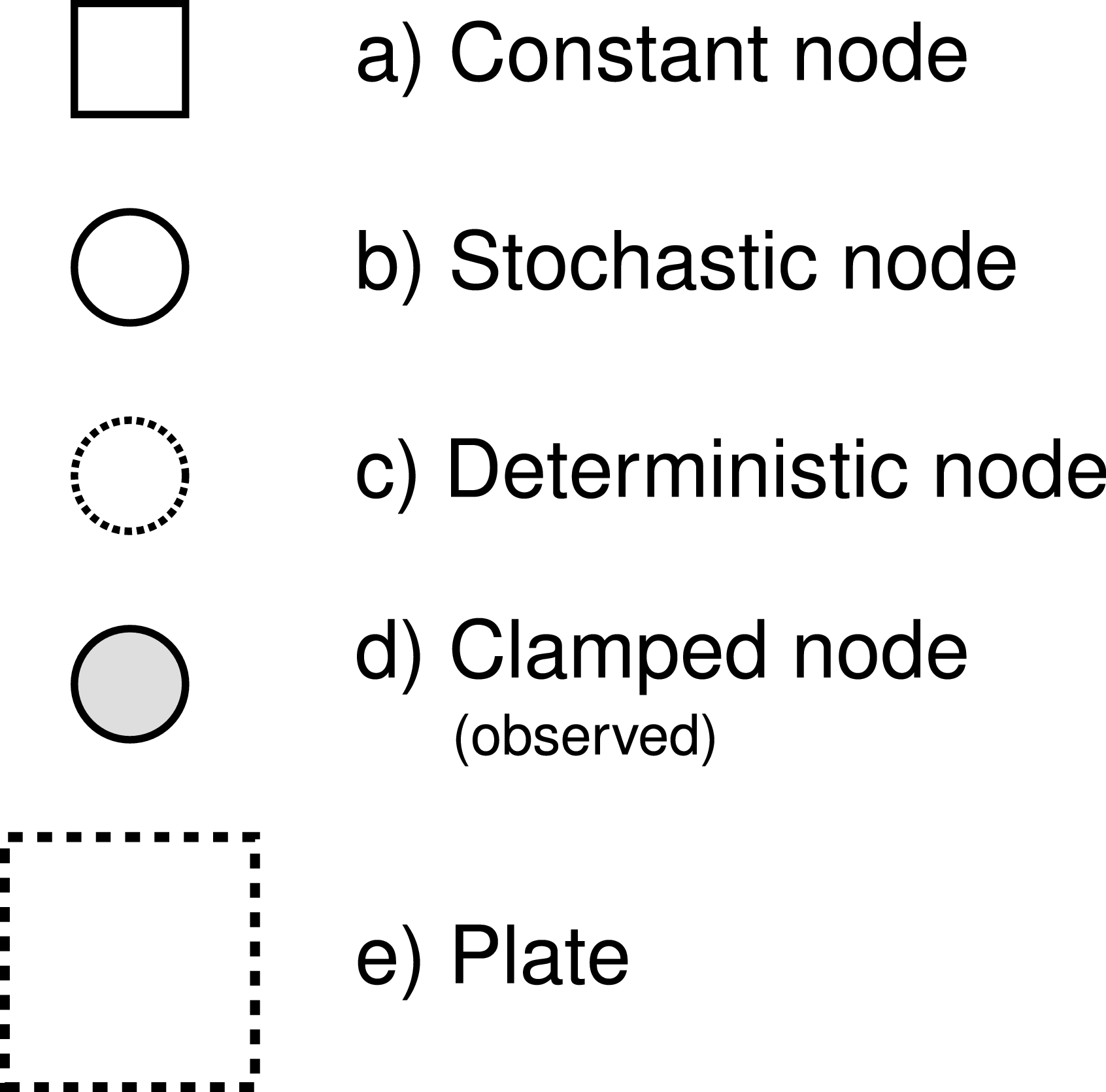
RevBayes uses probabilistic graphical models for model specification, visualization, and implementation (Höhna et al. 2014). Graphical models are frequently used in machine learning and statistics to conceptually represent the conditional dependence structure of complex statistical models with many parameters (missing reference). The graphical model framework allows for flexible model specification and implementation and reduces redundant code. This framework provides a set of symbols for depicting a directed acyclic graph (DAG). Höhna et al. (2014) described the use of probabilistic graphical models for phylogenetics. The different nodes and components of a phylogenetic graphical model are shown in [Fig. 1 from Höhna et al. (2014)].

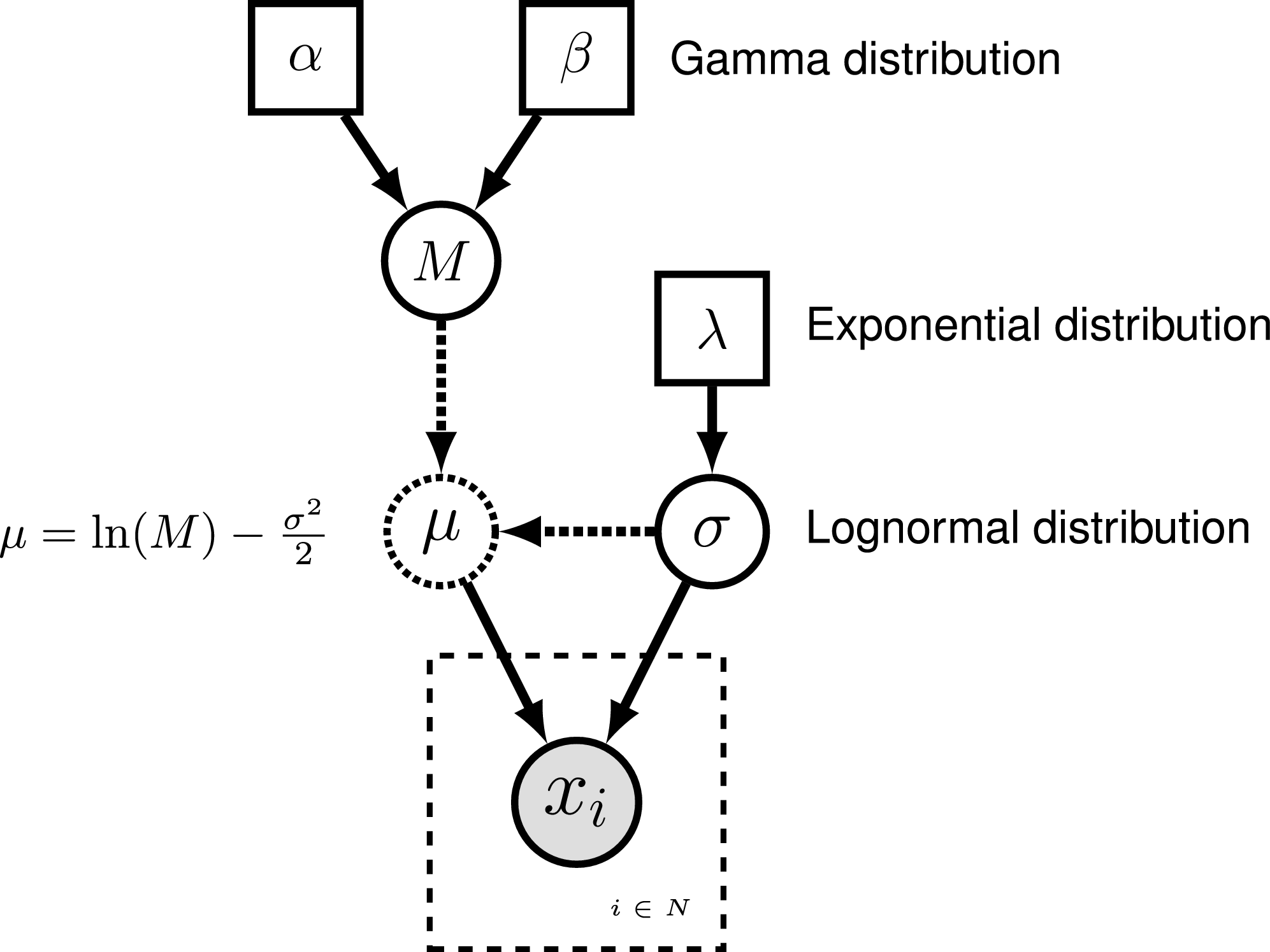
To represent the DAG, nodes are connected with arrows indicating dependency. A simple, albeit abstract, graphical model is shown in . In this model, we observe a set of states for parameter $x$. We assume that the values of $x$ are samples from a lognormal distribution with a location parameter (log mean) $\mu$ and a standard deviation $\sigma$. It is more straightforward to model our uncertainty in the expectation of a lognormal distribution, rather than $\mu$, thus we place a gamma distribution on the mean $M$. This gamma hyperprior has two parameters that we specify with fixed values (constant nodes): the shape $\alpha$ and rate $\beta$. The variable $M$ is a stochastic node with this prior density. The standard deviation, $\sigma$, is also a stochastic node with an exponential prior density with rate parameter $\lambda$. For any value of $M$ and any value of $\sigma$ we can compute the deterministic variable $\mu$ using the formula $\mu = \ln(M) - \frac{\sigma^2}{2}$. This formula is known from using simple algebra on the equation for the mean of any lognormal distribution. With this model structure, we can then calculate the probability of the data conditional on the model and parameter values (the likelihood): $\mathbb{P}(\boldsymbol{x} \mid \mu, \sigma)$. Next we can get the posterior probability using Bayes’ theorem: \(\mathbb{P}(M,\sigma \mid \boldsymbol{x}, \alpha, \beta, \lambda) = \frac{\mathbb{P}(\boldsymbol{x} \mid \mu, \sigma) \mathbb{P}(M \mid \alpha,\beta) \mathbb{P}(\sigma \mid \lambda)}{\mathbb{P}(\boldsymbol{x})}.\)

Rev: The RevBayes Language

In RevBayes models and analyses are specified using an interpreted language called Rev. Rev bears similarities to the compiled language in WinBUGS and the interpreted Rlanguage. Setting up and executing a statistical analysis in RevBayes requires the user to specify all of the parameters of their model and the type of analysis (e.g.,an MCMC run). By using an interpreted language, RevBayes enables the practitioner to build complex, hierarchical models and to check the current states of variables while building the model. This will be very useful in the beginning. Later on you, when you run very complex analyses, you may want to write Rev-scripts.

Differently to Rand BUGS, Rev is a strongly but implicitly typed language. It is implicitly typed, and thus similar to Python, because you do not need to provide the type of a variable (which you need to in languages such as C++ and Java). We do implicit typing to help users who do not know about the actual types of the variables. However, strongly typed means that every variable has a type and arguments of functions need to match the required types. The strong type requirements ensures that you build meaningful model graphs. For example, the variance parameter of a normal distribution needs to be a positive number, and thus you can only use variables that are positive real numbers. RevBayes does automatic type conversion.

Specifying Models

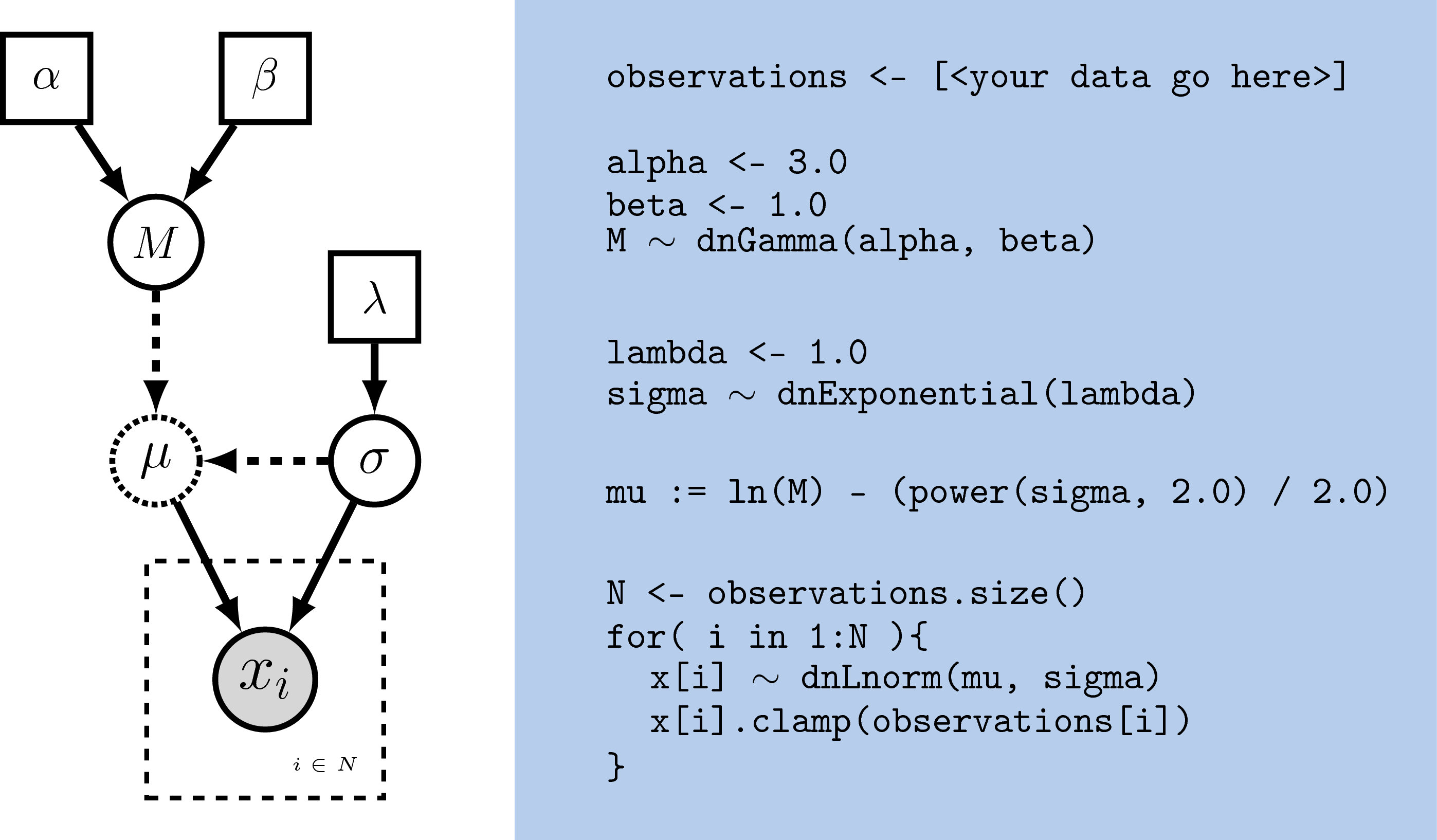
The variables/parameters of a statistical model are created using different operators in Rev (). In Figure [revgmexample], the Rev syntax for creating the model in Figure [simpleGM] is provided. Because Rev is an interpreted language, it is important to consider the order in which you specify your variables (cf.BUGS where the order is not important). Thus, typically the first variables that are instantiated are constant variables. Constant variables require you to assign a fixed value using the <- operator. Stochastic variables are initialized using the ~ operator followed by the constructor function for a distribution. In Rev, the naming convention for distributions is dn*, where * is a wildcard representing the name of the distribution. Each distribution function requires hyperparameters passed in as arguments. This is effectively linking nodes using arrows in the graphical model. The following code snippet creates a stochastic variable called M which is assigned a gamma-distributed hyperprior, with shape alpha and rate beta:

alpha <- 2.0
beta <- 4.0
M ~ dnGamma(alpha, beta)

The flexibility gained from the graphical model framework and the interpreted language allows you to easily change a model by swapping components. For example, if you decide that a bimodal lognormal distribution is a better representation of your uncertainty in M, then you can simply change the distribution associated with M (after initializing the bimodal lognormal hyperparameters):

mean_1 <- 0.5
mean_2 <- 2.0
sd_1 <- 1.0
sd_2 <- 1.0
weight <- 0.5
M ~ dnBimodalLognormal(mean_1, mean_2, sd_1, sd_2, weight)

Rev does allow you to specify constant-variable values in the distribution constructor function; therefore this also works:

M ~ dnBimodalLognormal(0.5, 2.0, 1.0, 1.0, 0.5)

Both ways to specify priors are equivalent. The only difference is that one code may be more readable than the other.

Deterministic variables are parameter transformations and initialized using the := operator followed by the function or formula for calculating the value. Previously we created a variable for the expectation of the lognormal distribution. Now, if you have an exponentially distributed stochastic variable $\sigma$, you can create a deterministic variable for the mean $\mu$:

lambda <- 1.0
sigma ~ dnExponential(lambda)
mu := ln(M) - (sigma^2)/2.0

Replication over lists of variables as a plate object is specified using for loops. A for-loop is an iterator statement that performs a function a given number of times. In Rev you can use this syntax to create a vector of 7 stochastic variables, each drawn from a lognormal distribution:

for( i in 1:7 ) {
   x[i] ~ dnLognormal(mu, sigma)
}

The for loop executes the statement x[i] ~ dnLognormal(mu, sigma) for different values of $i$ repeatedly, where $i$ takes the values 1 to 7. Thus, we created a vector $x$ of seven variables, each being independent and identically distributed (i.i.d.).

A clamped node/variable has observed data attached to it. Thus, you must first read in or input the data, then clamp it to a stochastic variable. In the observations are assigned and clamped to the stochastic variables. If we observed 7 values for $x$ we would create 7 clamped variables:

observations <- [0.20, 0.21, 0.03, 0.40, 0.65, 0.87, 0.22]
N <- observations.size()
for( i in 1:N ){
   x[i].clamp(observations[i])
}

You may notice that the value of $x$ has now changed and is equal to the observations.

Getting help in RevBayes

RevBayes provides an elaborate help system. Most of the help is found online on our website. Within RevBayes you can display the help for a function, distribution or any other type using the ? symbol followed by the command you want help for:

?dnNorm
?mcmc
?mcmc.run

Additionally, RevBayes will print the correct usage of a function if you only type in its name and hit return:

mcmc

       MCMC function (Model model, Monitor[] monitors, Move[] moves, String moveschedule = "sequential" | "random" | "single", Natural nruns)

RevBayes Users’ Forum

An email list has been created for users of RevBayes to discuss RevBayes-related topics, including: RevBayes installation and use, scripting and programming, phylogenetics, population genetics, models of evolution, graphical models, etc. The forum is hosted by Google Groups: revbayes-users

1. Höhna S., Landis M.J., Heath T.A., Boussau B., Lartillot N., Moore B.R., Huelsenbeck J.P., Ronquist F. 2016. RevBayes: Bayesian Phylogenetic Inference Using Graphical Models and an Interactive Model-Specification Language. Systematic Biology. 65:726–736. 10.1093/sysbio/syw021
2. Höhna S., Heath T.A., Boussau B., Landis M.J., Ronquist F., Huelsenbeck J.P. 2014. Probabilistic Graphical Model Representation in Phylogenetics. Systematic Biology. 63:753–771. 10.1093/sysbio/syu039