Basic Rev Commands
This tutorial demonstrates the basic syntactical features of RevBayes and the Rev scripting language. A good reference for probabilistic graphical models for Bayesian phylogenetic inference is given in (Höhna et al. 2014). Let’s start with the basic concepts for the interactive use of RevBayes with Rev (the language of RevBayes). You should try to execute the statements step by step, look at the output and try to understand what and why things are happening.
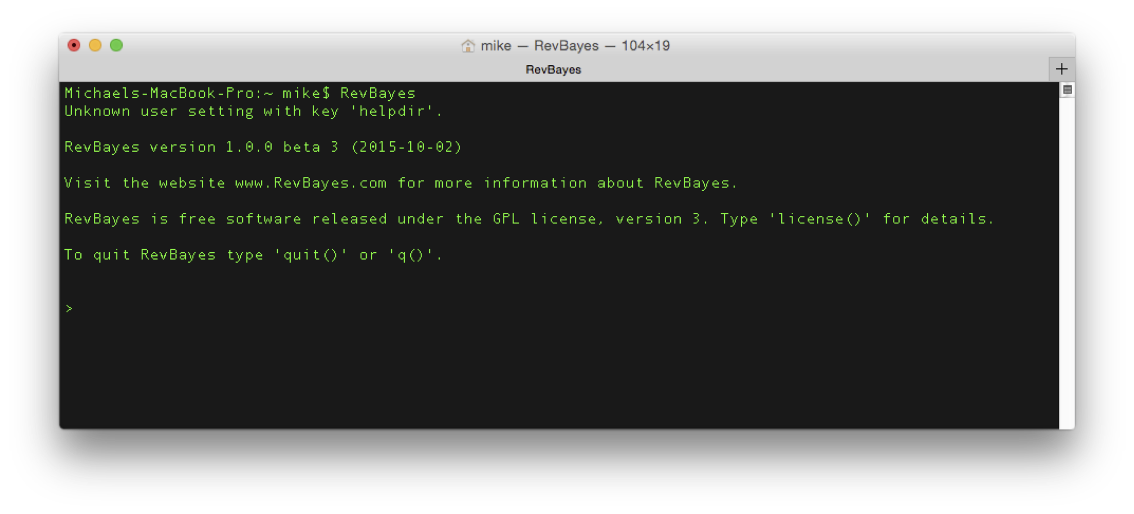
First, open up your terminal and type RevBayes. This should launch RevBayes and give you
a command prompt (the > character). This means RevBayes is waiting for input.
Operators and Functions
Rev is an interpreted language for statistical computing and phylogenetic analysis. Therefore, the basics are simple mathematical operations. Entering each of the following lines will automatically execute these operations.
# Simple mathematical operators:
1 + 1                            # Addition
10 - 5                           # Subtraction
5 * 5                            # Multiplication
10 / 2                           # Division
2^3                              # Exponentiation
5%2                              # Modulo
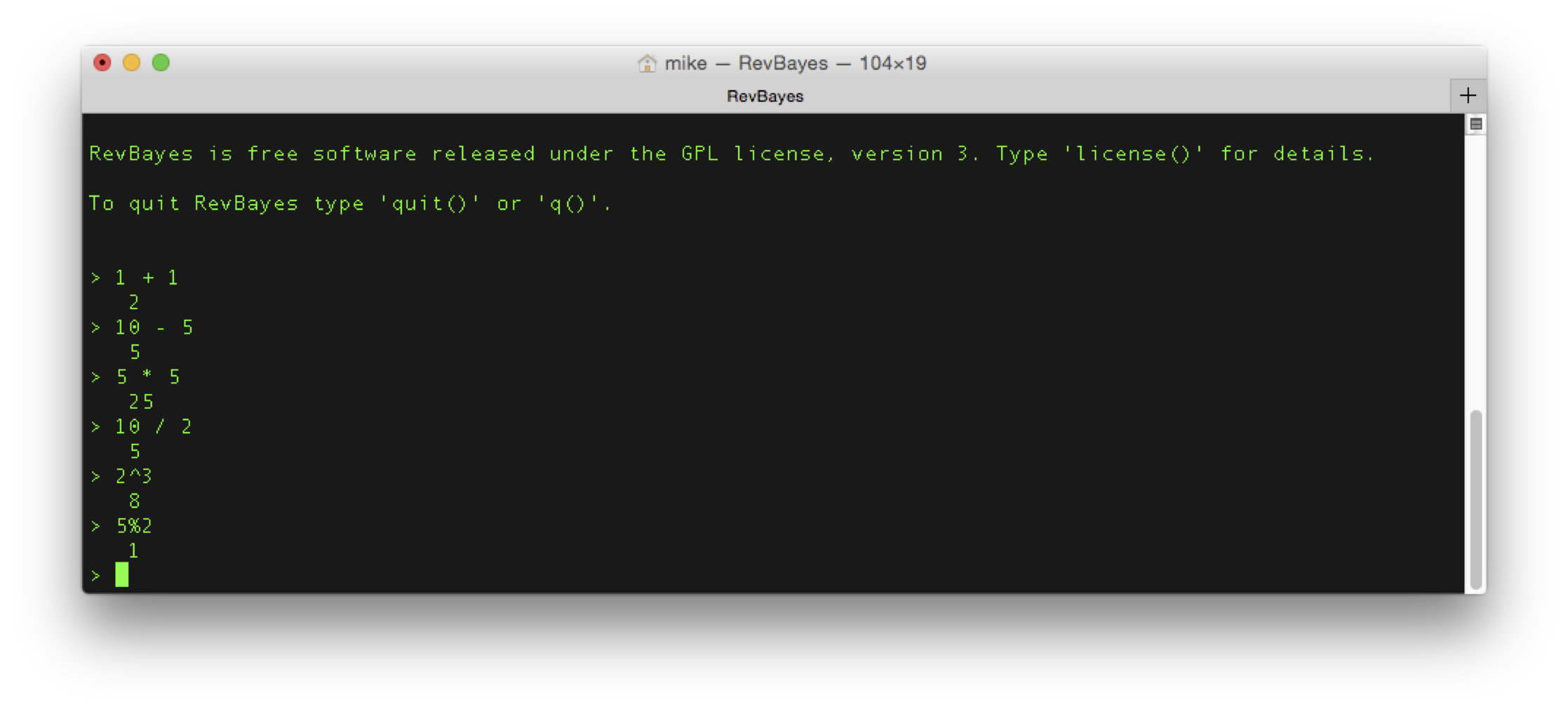
From now on, we will omit images of the terminal.
Each set of operations constitutes a statement. As you work through these tutorials, it is helpful to write the statements you enter into a blank text file, then copy-and-paste the statements into to execute them. This way, you have a complete history of everything you’ve done, and can easily start over without having to rewrite everything. We refer to the text file containing the list of commands as a script, because it describes line-by-line instructions for the program to follow.
You can write multiple statements in the same line if you separate them
by a semicolon (;). The statements will execute as if you wrote each
on a single line.
1 + 1; 2 + 2 # Multiple statements in one line
Here you can see that comments always start with the hash symbol (#).
Everything after the #-symbol will be ignored. In addition to these
simple mathematical operations, provides some standard math functions
which can be called by:
# Math functions
exp(1)                           # exponential function
ln(1)                            # logarithmic function with natural base
sqrt(16)                         # square root function
power(2,2)                       # power function: power(a,b) = a^b
Notice that Rev is case-sensitive. That means, Rev distinguishes upper and lower case letter for both variable names and function names. For example, only the first of these two calls will work:
exp(1)                           # correct lower case name
Exp(1)                           # wrong upper case name
Variable Declaration and Assignment
One of the most important features of (or any programming language, really) is the ability to declare and assign variables. Variables store information to be referenced later, and can change throughout the execution of the program. There are three kinds of variables in RevBayes, called constant, deterministic, and stochastic variables. Constant variables contain values that are not random in your model. Deterministic variables are functions of other variables. Stochastic variables are random variables in your model, and will change during your analysis; importantly, stochastic variables (being random variables) are always associated with a particular statistical distribution.
Different types of variables differ in how you create them and assign
values to them. We will begin by creating a constant variable with name
a that starts with the value 1. The left arrow assignment (<-)
always creates a constant variable, and automatically assigns the
following value to it.
# Variable assignment: constant
a <- 1                           # assignment of constant node `a'
You see the value of ‘a’ by just typing in the variable name and pressing enter.
a # printing the value of `a'
Next, we create a deterministic variable b using the := assignment
computed by exp(a) and another deterministic variable c computed by
ln(b). Deterministic variables are always created using the
colon-equal assignment (:=).
# Variable assignment: deterministic

# assignment of deterministic node `b' with
# the exponential function with parameter `a'
b := exp(a)
b

# assignment of deterministic node `c' with
# logarithmic function with parameter `b'
c := ln(b)
c
Finally, we will create the third type of variables in RevBayes: stochastic
variables. We will create a random variable x from an exponential
distribution with parameter lambda. Stochastic assignments use the
$\sim$ operation.
# Variable assignment: stochastic

# assign constant node `lambda' with value `1'
lambda <- 1.0

# create stochastic node with exponential
# distribution and parameter `lambda'
x ~ dnExponential(lambda)
The value of x is a random draw from the distribution. You can see the
value and the probability (or log-probability) of the current value
under the current parameter values by
x                                # print value of stochastic node `x'
x.probability()                  # print the probability if `x'
x.lnProbability()                # print the log-probability if `x'
Distributions and Random Numbers
RevBayes provides functions for common statistical distributions. We’ll demonstrate by generating random exponential numbers as we did in lecture. Recall that we can transform a random variable $u$ sampled from a Uniform(0,1) distribution into an exponential distribution with rate parameter $\lambda$:
\[\begin{aligned} u &\sim \text{Uniform(0,1)}\\ x &= -\frac{\ln u}{\lambda} \end{aligned}\]In RevBayes, we might describe $u$ as a stochastic variable, and $x$ as a deterministic variable (since it is a function of $u$):
# create the random variable u
u ~ dnUniform(0,1)
u

# determine the rate parameter
lambda <- 1.0

# create x as a deterministic function of u
x := -ln(u) / lambda
x
Alternatively, we can create $x$ directly as an exponential random variable:
# create the random variable x
x ~ dnExponential(lambda)
x
Vectors
Individual variables can have more than one value. Variables that have more than one value are called vectors. The simplest way to create a vector is like this:
z <- v(1.0,2.0,3.0) # create a vector
You can refer to a specific value in the vector using brackets, [i],
where i is the index of the variable of interest.
z[1]                             # print the first entry
z[1] <- 10                       # change the value of the first entry
z
for loops
for loops are important programming structures that allow you to
repeat the same statement a number of times on different variables. The
basic structure of a for loop is:
# a for loop
for ([variable] in [set of values]) {
   [statements using variable]
}
The for statement is followed by a set of parenthesis containing
[variable], which contains the name of the variable being iterated,
and [set of values], which are the values that the variable iterates
over. The for loop variable is a special variable that is created by
the for loop: you do not have to create it before executing the loop.
This simple for loop creates the variable i, and for each value of
i from 1 to 100, prints the value of i to the screen.
for (i in 1:100) {
   i
}
for loops are very powerful programming tools. We can use a for loop
to create an entire vector of uniform random numbers, and transform
them into a second vector of exponential random numbers.
for (i in 1:100) {
   y[i] ~ dnUniform(0,1)
   z[i] := -ln(y[i]) / lambda
}
Close using the statement q().
q()
- Höhna S., Heath T.A., Boussau B., Landis M.J., Ronquist F., Huelsenbeck J.P. 2014. Probabilistic Graphical Model Representation in Phylogenetics. Systematic Biology. 63:753–771. 10.1093/sysbio/syu039