Overview

This very basic tutorial provides an introduction to Bayesian inference and Markov chain Monte Carlo (MCMC) algorithms. The tutorial explains the fundamental concepts of an MCMC algorithm, such as moves and monitors, which are ubiquitous in every other tutorial. After the tutorial you should be somewhat familiar with Bayesian inference (e.g., what is a prior distribution, posterior distribution, and likelihood function) and MCMC simulation (e.g., what are moves and monitors and why do we need them).

This tutorial comes with a recorded video walkthrough. The video corresponding to each section of the exercise is linked next to the section title. The full playlist is available here:

A Coin Flipping (Binomial) Model

We’ll begin our exploration of Bayesian inference with a simple coin-flipping model. In this model, we imagine flipping a coin $n$ times and count the number of heads, $x$; each flip comes up heads with probability $p$. This model gives rise to the Binomial probability distribution, with parameters $n$ and $p$: \(\begin{aligned} P(x \mid n,p) = {n \choose x}p^x(1-p)^{n-x}\end{aligned}\) Simple intuition suggests that, given that we observe $x$ heads in $n$ coin tosses, the maximum-likelihood estimate (MLE) of $p$ is simply $\frac{x}{n}$: if we flip a coin 100 times and observe 70 heads, we assume the probability the coin comes up heads is $\frac{70}{100} = 0.7$. This is indeed the maximum likelihood estimate!

From Bayes’ theorem, the posterior distribution of $p$ given $x$, $P(p \mid x)$, is: \(\begin{aligned} \overbrace{P(p \mid x)}^{\text{posterior distribution}} = \frac{\overbrace{P(x \mid p)}^{\text{likelihood}} \times \overbrace{P(p)}^{\text{prior}}}{\underbrace{P(x)}_{\text{marginal likelihood}}} \end{aligned}\) The take-home message here is that if we’re interested in doing Bayesian inference for the coin flipping model, we need to specify a likelihood function and a prior distribution for $p$. In virtually all practical cases, we cannot compute the posterior distribution directly and instead use numerical procedures, such as a Markov chain Monte Carlo (MCMC) algorithm. Therefore, we will also have to write an MCMC algorithm that samples parameter values in the frequency of their posterior probability.

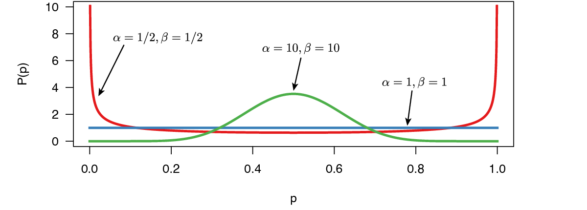
We’ll use a simple beta distribution as a prior on the parameter of the model, $p$. The beta distribution has two parameters, $\alpha$ and $\beta$ (). Different choices for $\alpha$ and $\beta$ represent different prior beliefs.

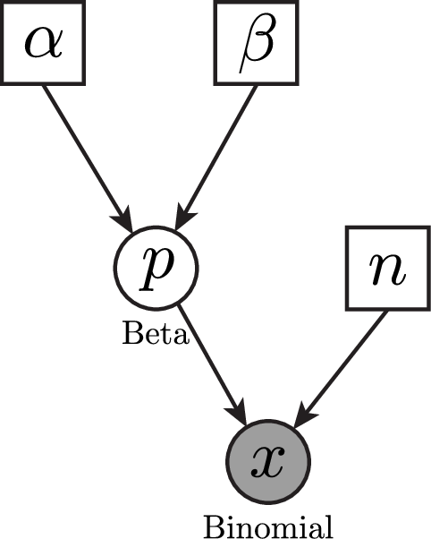
shows the graphical model for the binomial model. This nicely visualizes the dependency structure in the model. We see that the two parameters $\alpha$ and $\beta$ are drawn in solid squares, representing that these variables are constant. From these two variables, we see arrows going into the variable $p$. That simply means that $p$ depends on $\alpha$ and $\beta$. More specifically, $p$ is a stochastic variable (shown as a solid circle) and drawn from a beta distribution with parameters $\alpha$ and $\beta$. Then, we have another constant variable, $n$. Finally, we have the observed data $x$ which is drawn from a Binomial distribution with parameters $p$ and $n$, as can be seen by the arrows going into $x$. Furthermore, the solid circle of $x$ is shaded which means that the variable has data attached to it.

Writing an MCMC from Scratch

Make yourself familiar with the example script called Binomial_MH_algorithm.Rev which shows the code for the following sections. Then, start a new and empty script and follow each step provided in this tutorial.

The Metropolis-Hastings Algorithm

Though RevBayes implements efficient and easy-to-use Markov chain Monte Carlo algorithms, we’ll begin by writing one ourselves to gain a better understanding of the moving parts. The Metropolis-Hastings MCMC algorithm (missing reference) proceeds as follows:

1. Generate initial values for the parameters of the model (in this case, $p$).

2. Propose a new value (which we’ll call $p^\prime$) for some parameters of the model, (possibly) based on their current values

3. Calculate the acceptance probability, $R$, according to: \(\begin{aligned} R = \text{min}\left\{1, \frac{P(x \mid p^\prime)}{P(x \mid p)} \times \frac{P(p^\prime)}{P(p)} \times \frac{q(p)}{q(p^\prime)} \right\} \end{aligned}\)

4. Generate a uniform random number between 1 and 0. If it is less than $R$, accept the move (set $p = p^\prime$). Otherwise, keep the current value of $p$.

5. Record the values of the parameters.

6. Return to step 2 many many times, keeping track of the value of $p$.

Reading in the data

Actually, in this case, we’re just going to make up some data on the spot. Feel free to alter these values to see how they influence the posterior distribution

    # Make up some coin flips!
    # Feel free to change these numbers
    n <- 100 # the number of flips
    x <- 63	# the number of heads

Initializing the Markov chain —————————–

We have to start the MCMC off with some initial parameter values. One way to do this is to randomly draw values of the parameters (just $p$, in this case) from the prior distribution. We’ll assume a “flat” beta prior distribution; that is, one with parameters $\alpha = 1$ and $\beta = 1$.

    # Initialize the chain with starting values
    alpha <- 1
    beta  <- 1
    p <- rbeta(n=1,alpha,beta)[1]

Likelihood function

We also need to specify the likelihood function. We use the binomial probability for the likelihood function. Since the likelihood is defined only for values of $p$ between 0 and 1, we return 0.0 if $p$ is outside this range:

    # specify the likelihood function
    function likelihood(p) {
        if(p < 0 || p > 1)
            return 0

        l = dbinomial(x,p,n,log=false)
        return l
    }

Prior distribution

Similarly, we need to specify a function for the prior distribution. Here, we use the beta probability distribution for the prior on $p$:

    # specify the prior function
    function prior(p) {
        if(p < 0 || p > 1)
            return 0

        pp = dbeta(p,alpha,beta,log=false)
        return pp
    }

Monitoring parameter values

Additionally, we are going to monitor, i.e., store, parameter values into a file during the MCMC simulation. For this file we need to write the column headers:

    # Prepare a file to log our samples
    write("iteration","p","\n",file="binomial_MH.log")
    write(0,p,"\n",file="binomial_MH.log",append=TRUE)

(You may have to change the newline characters to \backslashr\backslashn if you’re using a Windows operating system.) We’ll also monitor the parameter values to the screen, so let’s print the initial values:

    # Print the initial values to the screen
    print("iteration","p")
    print(0,p)

Writing the MH Algorithm ————————

At long last, we can write our MCMC algorithm. First, let us define the frequency how often we print to file (i.e., monitor), which is also often called thinning. If we set the variable printgen to 1, then we will store the parameter values every single iteration; if we choose printgen=10 instead, then only every $10^{th}$ iteration.

    printgen = 10

We will repeat this resampling procedure many times (here, 10000), and iterate the MCMC using a for loop:

    # Write the MH algorithm
    reps = 10000
    for(rep in 1:reps){

(remember to close your for loop at the end).

The first thing we do in the first generation is generate a new value of $p^\prime$ to evaluate. We’ll propose a new value of $p$ from a uniform distribution between 0 and 1. Note that in this first example we do not condition new parameter values on the current value.

    	# Propose a new value of p
    	p_prime <- runif(n=1,0.0,1.0)[1]

Next, we compute the proposed likelihood and prior probabilities, as well as the acceptance probability, $R$:

    	# Compute the acceptance probability
    	R <- ( likelihood(p_prime) / likelihood(p) ) * ( prior(p_prime) / prior(p) )

Then, we accept the proposal with probability $R$ and reject otherwise:

    	# Accept or reject the proposal
    	u <- runif(1,0,1)[1]
    	if(u < R){
    		# Accept the proposal
    		p <- p_prime
    	}

Finally, we store the current value of $p$ in our log file. Here, we actually check if we want to store the value during this iteration.

        if ( (rep % printgen) == 0 ) {
            # Write the samples to a file
            write(rep,p,"\n",file="binomial_MH.log",append=TRUE)
            # Print the samples to the screen
            print(rep,p)
        }
    } # end MCMC

Visualizing the samples of an MCMC simulation ———————————————

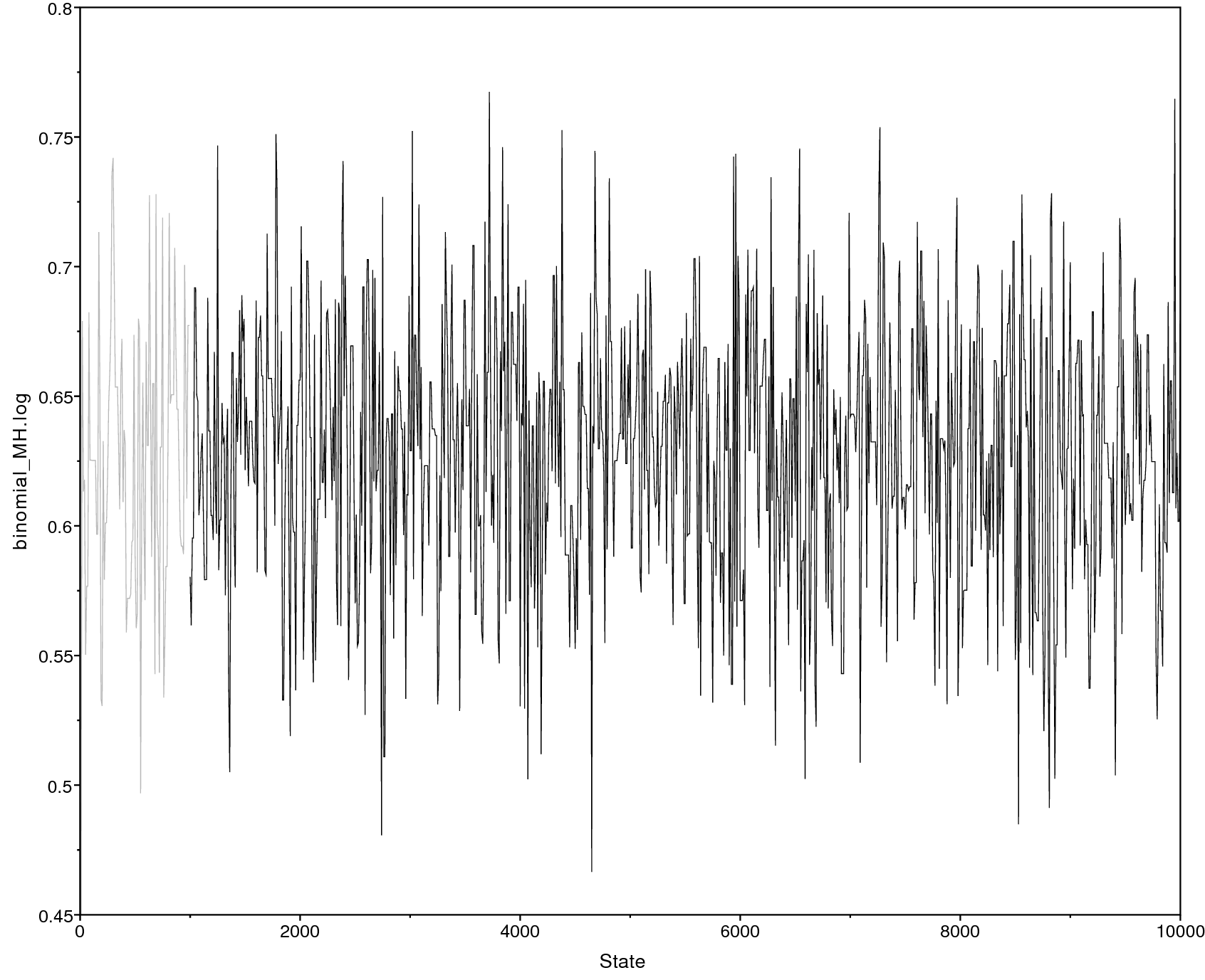
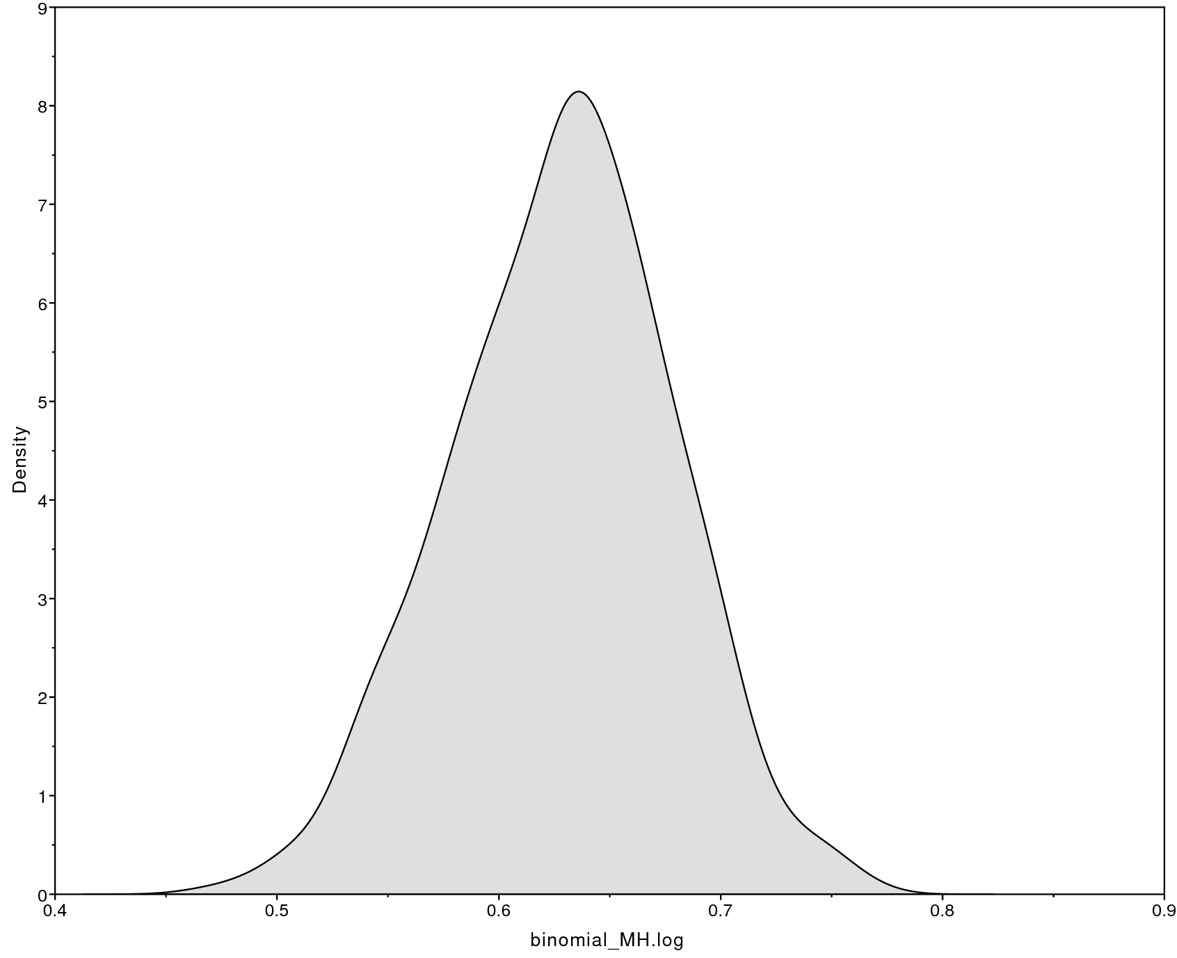
Below we show an example of the obtained output in Tracer. Specifically, shows the sample trace (left) and the estimated posterior distribution of $p$ (right). There are other parameters, such as the posterior mean and the 95% HPD (highest posterior density) interval, that you can obtain from Tracer.

More on Moves: Tuning and weights

In the previous example we hard coded a single move updating the variable $p$ by drawing a new value from a uniform(0,1) distribution. There are actually many other ways how to propose new values; some of which are more efficient than others.

First, let us rewrite the MCMC loop so that we use instead a function, which we call move_uniform for simplicity, that performs the move:

    for (rep in 1:reps){

        # call uniform move
        move_uniform(1)

        if ( (rep % printgen) == 0 ) {
            # Write the samples to a file
            write(rep,p,"\n",file="binomial_MH.log",append=TRUE)
        }

    } # end MCMC

This loop looks already much cleaner.

Uniform move

Now we need to actually write the move_uniform function. We mostly just copy the code we had before into a dedicated function

    function move_uniform( Natural weight) {

        for (i in 1:weight) {
            # Propose a new value of p
            p_prime <- runif(n=1,0.0,1.0)[1]

            # Compute the acceptance probability
            R <- ( likelihood(p_prime) / likelihood(p) ) * ( prior(p_prime) / prior(p) )

            # Accept or reject the proposal
            u <- runif(1,0,1)[1]
            if (u < R){
                # Accept the proposal
                p <- p_prime
            } else {
                # Reject the proposal
                # (we don't have to do anything here)
            }
        }

    }

There are a few things to consider in the function move_uniform. First, we do not have a return value because the move simply changes the variable $p$ if the move is accepted. Second, we expect an argument called weight which will tell us how often we want to use this move. Otherwise, this function does exactly the same what was inside the for loop previously.

(Note that you need to define this function before the for loop in your script).

Sliding-window move

As a second move we will write a sliding-window move. The sliding-window moves propose an update by drawing a random number from a uniform distribution and then adding this random number to the current value (i.e., centered on the previous value).

    function move_slide( RealPos delta, Natural weight) {

        for (i in 1:weight) {
            # Propose a new value of p
            p_prime <- p + runiform(n=1,-delta,delta)[1]

            # Compute the acceptance probability
            R <- ( likelihood(p_prime) / likelihood(p) ) * ( prior(p_prime) / prior(p) )

            # Accept or reject the proposal
            u <- runif(1,0,1)[1]
            if (u < R) {
                # Accept the proposal
                p <- p_prime
            } else {
                # Reject the proposal
                # (we don't have to do anything here)
            }
        }

    }

In addition to the weight of the move, this move has another argument, delta. The argument delta defines the width of the uniform window from which we draw new values. Thus, if delta is large, then the proposed values are more likely to be very different from the current value of $p$. Conversely, if delta is small, then the proposed values are more likely to be very close to the current value of $p$.

Experiment with different values for delta and check how the effective sample size (ESS) changes.

There is, a priori, no good method for knowing what values of delta are most efficient. However, there are some algorithms implemented in RevBayes, called auto-tuning, that will estimate good values for delta.

Scaling move

As a third and final move we will write a scaling move. The scaling move proposes an update by drawing a random number from a uniform(-0.5,0.5) distribution, exponentiating the random number, and then multiplying this scaling factor by the current value. An interesting feature of this move is that it is not symmetrical and thus needs a Hastings ratio. The Hastings ratio is rather trivial in this case, and one only needs to multiply the acceptance rate by the scaling factor.

    function move_scale( RealPos lambda, Natural weight) {

        for (i in 1:weight) {
            # Propose a new value of p
            sf <- exp( lambda * ( runif(n=1,0,1)[1] - 0.5 ) )
            p_prime <- p * sf

            # Compute the acceptance probability
            R <- ( likelihood(p_prime) / likelihood(p) ) * ( prior(p_prime) / prior(p) ) * sf

            # Accept or reject the proposal
            u <- runif(1,0,1)[1]
            if (u < R){
                # Accept the proposal
                p <- p_prime
            } else {
                # Reject the proposal
                # (we don't have to do anything here)
            }
        }

    }

As before, this move has a tuning parameter called lambda.

The sliding-window and scaling moves are very common and popular moves in RevBayes. The code examples here are actually showing the exact same equation as implemented internally. It will be very useful for you to understand these moves.

However, this MCMC algorithm is very specific to our binomial model and thus hard to extend (also it’s pretty inefficient!).

The Metropolis-Hastings Algorithm with the Real RevBayes

The video walkthrough for this section is in two parts. Part 1 Part 2

We’ll now specify the exact same model in Rev using the built-in modeling functionality. It turns out that the Rev code to specify the above model is extremely simple and similar to the one we used before. Again, we start by “reading in” (i.e., making up) our data.

    # Make up some coin flips!
    # Feel free to change these numbers
    n <- 100 # the number of flips
    x <- 63	# the number of heads

Now we specify our prior model.

    # Specify the prior distribution
    alpha <- 1
    beta  <- 1
    p ~ dnBeta(alpha,beta)

One difference between RevBayes and the MH algorithm that we wrote above is that many MCMC proposals are already built-in, but we have to specify them before we run the MCMC. We usually define (at least) one move per parameter immediately after we specify the prior distribution for that parameter.

    # Define a move for our parameter, p
    moves[1] = mvSlide(p,delta=0.1,weight=1)

Next, our likelihood model.

    # Specify the likelihood model
    k ~ dnBinomial(p, n)
    k.clamp(x)

We wrap our full Bayesian model into one model object (this is a convenience to keep the entire model in a single object, and is more useful when we have very large models):

    # Construct the full model
    my_model = model(p)

We use “monitors” to keep track of parameters throughout the MCMC. The two kinds of monitors we use here are the mnModel, which writes parameters to a specified file, and the mnScreen, which simply outputs some parts of the model to screen (as a sort of progress bar).

    # Make the monitors to keep track of the MCMC
    monitors[1] = mnModel(filename="binomial_MCMC.log", printgen=10, separator = TAB)
    monitors[2] = mnScreen(printgen=100, p)

Finally, we assemble the analysis object (which contains the model, the monitors, and the moves) and execute the run using the .run command:

    # Make the analysis object
    analysis = mcmc(my_model, monitors, moves)

    # Run the MCMC
    analysis.run(100000)

    # Show how the moves performed
    analysis.operatorSummary()

Open the resulting binomial_MCMC.log file in Tracer. Do the posterior distributions for the parameter $p$ look the same as the ones we got from our first analysis?

Hopefully, you’ll note that this Rev model is substantially simpler and easier to read than the MH algorithm script we began with. Perhaps more importantly, this Rev analysis is orders of magnitude faster than our own script, because it makes use of extremely efficient probability calculations built-in to RevBayes (rather than the ones we hacked together in our own algorithm).

Exercises for the MCMC Tutorial

Exercise 1: Performing your first simple MCMC simulation

1. Look into the Binomial_MH_algorithm.Rev script and make yourself familiar with it. All the commands should be explained in the text of the tutorial.

2. Execute the script Binomial_MH_algorithm.Rev.

3. The .log file will contain samples from the posterior distribution of the model! Open the file in Tracerto learn about various features of the posterior distribution, for example: the posterior mean or the 95% credible interval.

4. Save the MCMC trace plot and posterior distribution into a PDF file.

Exercise 2: Different MCMC strategies (moves)

1. Now look into the script called Binomial_MH_algorithm_moves.Rev which shows the 3 different types of moves described in this tutorial.

2. Run the script to estimate the posterior distribution of $p$ again.

3. Look at the output in Tracer.

4. Use only a single move and set printgen=1. Which move has the best ESS?

5. How does the ESS change if you use a delta=10 for the sliding-window move?

6. Add to each move a counter variable that counts how often the move was accepted. For example:

               if (u < R){
                   # Accept the proposal
                   p <- p_prime
                   ++num_sliding_move_accepted
               }
   

7. Have a look at how the acceptance rate changes for different values of the tuning parameters.

Exercise 3: MCMC in RevBayes

1. Run the built-in MCMC (Binomial_MCMC.Rev) and compare the results to your own MCMC. Are the posterior estimates the same? Are the ESS values similar? Which script was the fastest?

2. Next, add a second move moves[2] = mvScale(p,lambda=0.1,tune=true,weight=1.0) just after the first one. Run the analysis again and compare it to the original one. Did the second move help with mixing?

3. Finally, run a pre-burnin using analysis.burnin(generations=10000,tuningInterval=200) just before you call analysis.run(100000). This will auto-tune the tuning parameters (e.g., delta and lambda) so that the acceptance ratio is between 0.4 and 0.5.

4. What are the tuned values for delta and lambda? Did the auto-tuning increase the ESS?

Exercise 4: Approximating the posterior distribution

Modify the script Binomial_MCMC.Rev. Assume you flipped a coin 100 times and got 34 heads. Run the MCMC for 100,000 generations, printing every 100 samples to the file.

1. What is the posterior mean estimate of p? The 95% credible interval?

2. Pretend you flipped the coin 900 more times, for a total of 1000 flips. Among those 1000 flips, you observed 340 heads (change your script accordingly!). What is your posterior mean estimate of p now? How has the 95% credible interval changed? Provide an intuitive explanation for this change.

Exercise 5: Exploring prior sensitivity and MCMC settings

Play around with various parts of the model to develop on intuition for both the Bayesian model and the MCMC algorithm. For example, how does the posterior distribution change as you increase the number of coin flips (say, increase both the number of flips and the number of heads by an order of magnitude)? How does the estimated posterior distribution change if you change the prior model parameters, $\alpha$ and $\beta$ (i.e., is the model prior sensitive)? Does the prior sensitivity depend on the sample size? Are the posterior estimates sensitive to the length of the MCMC? Do you think this MCMC has been run sufficiently long, or should you run it longer? Try to answer some of these questions and explain your findings.