Introduction
Example: Ancestral state estimation with a simple equal rates model
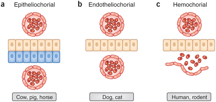
In this example we will look at the evolution of morphological character placenta type in placental mammals. We have three different types of placenta: Epitheliochorial(1), Endotheliochorial(2), Hemochorial(3) ( (PrabhuDas et al. 2015)). We are interested, in general, in the evolution of placenta type in placental mammals. Specifically, we want to know what the ancestral state of all placental mammals is. Furthermore, we want to know if placenta type is evolving under an equal-rates model, an unequal rates model, an irreversible model, or any other type of transition model.
Specifying the Mk Model
We will start this tutorial with the simple Mk model with three states, $k=3$ (Lewis 2001). Thus, we will follow the Discrete morphology - Tree Inference Tutorial very closely and refer you to that tutorial for more information.
Let us start with defining the rate matrix $Q$ for this 3-state model: \(Q = \begin{pmatrix} -\mu_1 & \mu_{12} & \mu_{13} \\ \mu_{21} & -\mu_2 & \mu_{23} \\ \mu_{31} & \mu_{32} & -\mu_3 \end{pmatrix} \mbox{ .}\)
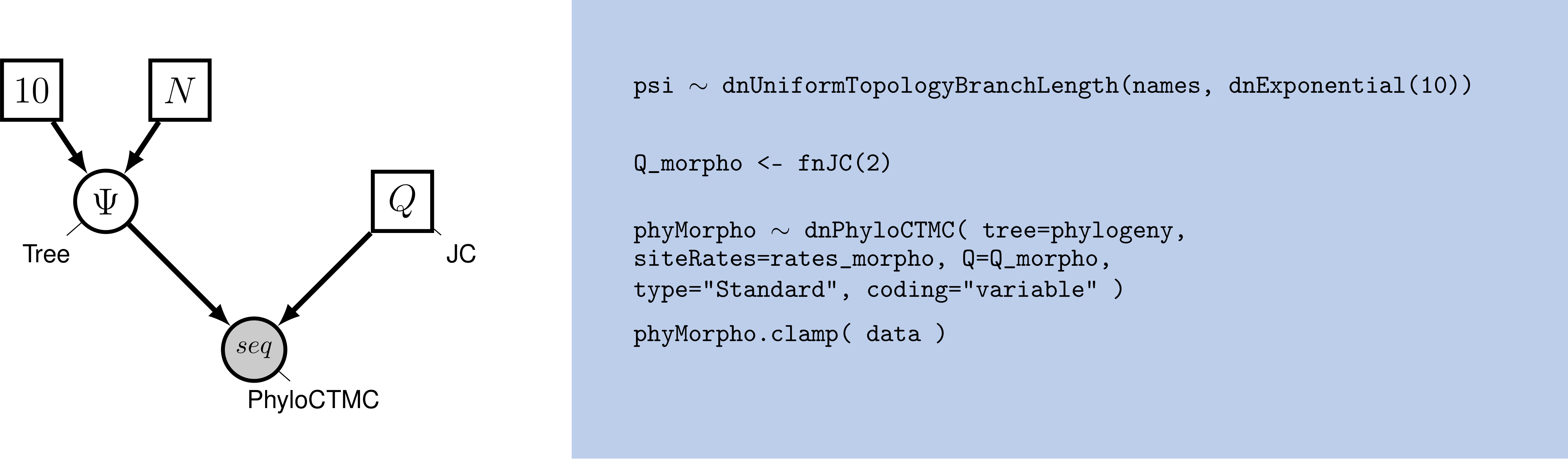
Remember, the Mk model sets transitions to be equal from any state to any other state. In that sense, our 3-state matrix really looks like this: \(Q = \begin{pmatrix} -(k-1)\mu & \mu & \mu \\ \mu & -(k-1)\mu & \mu \\ \mu & \mu & -(k-1)\mu \\ \end{pmatrix} \mbox{ .}\)
Because this is a Jukes-Cantor-like model (Jukes and Cantor 1969), state frequencies do not vary as a model parameter. A visualization of this simple model can be seen in .
We will first perform a phylogenetic analysis using the Mk model. In further sections, we will explore how to relax key assumptions of the Mk model.
Example: Ancestral State Estimation Using the Mk Model
In this example, we will use the placenta type data applied to a thinned phylogeny of placental mammals. We have thinned the phylogeny only so that it will run considerably fast for this tutorial. Our actual analysis uses the full dataset of $\sim 5000$ taxa.
Data and Files
Create a directory called
RB_DiscreteMorphology_RateASE_Tutorial(or any name you like).Make sure that you have the data files copied into a subdirectory called
data: .
Getting Started
Create a new directory (in
RB_DiscreteMorphology_RateASE_Tutorial) calledscripts`. (If you do not have this folder, please refer to the directions in section .)
When you execute RevBayes in this exercise, you will do so within the main directory you created (RB_DiscreteMorphology_RateASE_Tutorial).
Creating Rev Files
For complex models and analyses, it is best to create Rev script files that will contain all of the model parameters, moves, and functions.
In this exercise, you will work primarily in your text editor and create a set of files that will be easily managed and interchanged.
In this first section, you will write the following files from scratch and save them in the scripts directory:
mcmc_ase_mk.Rev: the Rev-script file that loads the data, specifies the model describing discrete morphological character change (binary characters), and specifies the monitors and MCMC sampler.
All of the files that you will create are also provided in the this RevBayes tutorial. Please refer to these files to verify or troubleshoot your own scripts.
Open your text editor and create the master Rev file called
mcmc_ase_Mk.Revin thescriptsdirectory.Enter the Rev code provided in this section in the new model file.
The file you will begin in this section will be the one you load into RevBayes when you have completed all of the components of the analysis.
In this section you will begin the file and write the Rev commands for loading in the taxon list and managing the data matrices.
Then, starting in section , you will move on to writing module files for each of the model components.
Once the model files are complete, you will return to editing mcmc_ase_Mk.Rev and complete the Rev script with the instructions given in section .
Load Data Matrices
RevBayes uses the function readDiscreteCharacterData() to load a data matrix to the workspace from a formatted file.
This function can be used for both molecular sequences and discrete morphological characters.
Import the morphological character matrix and assign it to the variable morpho.
morpho <- readDiscreteCharacterData("data/mammals_thinned_placenta_type.nex")
Create Helper Variables
Before we begin writing the Rev scripts for each of the model components, we need to instantiate a couple ``helper variables’’ that will be used by downstream parts of our model specification files. Create vectors of moves and monitors
moves = VectorMoves()
monitors = VectorMonitors()
The Mk Model
First, we read in the tree topology:
phylogeny <- readTrees("data/mammals_thinned.tree")[1]
Next, we will create a Q matrix.
Recall that the Mk model is simply a generalization of the JC model.
Therefore, we will create a 3x3 Q matrix using fnJC, which initializes $Q$-matrices with equal transition probabilities between all states.
Q_morpho <- fnJC(3)
Now that we have the basics of the model specified, we will specify the only parameter of the model, $\mu$. The parameter specifies all the rates of morphological evolution:
mu_morpho ~ dnExponential( 1.0 )
Since $\mu$ is a rate parameter, we will apply a scaling move to update it.
moves.append( mvScale(mu_morpho,lambda=1, weight=2.0) )
Lastly, we set up the CTMC. This should be familiar from the Nucleotide substitution models tutorial. We see some familiar pieces: tree and Q matrix. We also have two new keywords: data type and coding. The data type argument specifies the type of data - in our case, “Standard”, the specification for morphology.
phyMorpho ~ dnPhyloCTMC(tree=phylogeny, branchRates=mu_morpho, Q=Q_morpho, type="Standard")
phyMorpho.clamp(morpho)
All of the components of the model are now specified.
Complete MCMC Analysis
Create Model Object
We can now create our workspace model variable with our fully specified model DAG.
We will do this with the model() function and provide a single node in the graph (phylogeny).
mymodel = model(phylogeny)
The object mymodel is a wrapper around the entire model graph and allows us to pass the model to various functions that are specific to our MCMC analysis.
Specify Monitors and Output Filenames
The next important step for our Rev script file is to specify the monitors and output file names.
The first monitor we will create will monitor every named random variable in our model graph.
This will include every stochastic and deterministic node using the mnModel monitor.
In this case, it will only be our rate variable $\mu$.
It is still useful to specify the model monitor this way for later extensions of the model.
We will also name the output file for this monitor and indicate that we wish to sample our MCMC every 10 cycles.
monitors.append( mnModel(filename="output/mk.log", printgen=10) )
The second monitor we will add to our analysis will print information to the screen.
Like with mnFile we must tell mnScreen which parameters we’d like to see updated on the screen.
monitors.append( mnScreen(printgen=100) )
The third and final monitor might be new to you: the mnJointConditionalAncestralState monitor computes and writes the ancestral states to file.
monitors.append( mnJointConditionalAncestralState(tree=phylogeny,
                                                   ctmc=phyMorpho,
                                                   filename="output/mk.states.txt",
                                                   type="Standard",
                                                   printgen=1,
                                                   withTips=true,
                                                   withStartStates=false) )
The core arguments this monitor needs are a tree object (tree=phylogeny),
the phylogenetic model (ctmc=phyMorpho), an output filename (filename="output/mk.states.txt"),
the data type for the characters (type="Standard"), and the sampling frequency (printgen=10}.
The final argument, withTips=true, indicates that we do wish to record the tip states because we didn’t know all tip values and might be interested in the most plausible values.
The monitor will produce a joint sample of ancestral states, where every ancestral state is conditional on the drawn value of its parent node state (except for the root node),
storing the samples every 10 iterations to the file "output/mk.states.txt".
Viewing the states file, we see
Iteration	end_1	end_2	end_3	end_4	end_5	...
0	2	3	3	3	3	...
1	2	3	3	3	3	...
2	2	3	3	3	3	...
3	2	3	3	3	3	...
4	2	3	3	3	3	...
5	2	3	3	3	3	...
6	2	3	3	3	3	...
7	2	3	3	3	3	...
8	2	3	3	3	3	...
9	2	3	3	3	3	...
10	2	3	3	3	3	...
...
Set-Up the MCMC
Once we have set up our model, moves, and monitors, we can now create the workspace variable that defines our MCMC run.
We do this using the mcmc() function that simply takes the three main analysis components as arguments.
mymcmc = mcmc(mymodel, monitors, moves, nruns=2, combine="mixed")
The MCMC object that we named mymcmc has a member method called .run().
This will execute our analysis and we will set the chain length to 10000 cycles using the generations option.
mymcmc.run(generations=10000, tuningInterval=200)
Once our Markov chain has terminated, we will process the ancestral state samples. This function will compute the posterior probabilities of the ancestral states from the samples. Later we can visuallize our ancestral states.
anc_states = readAncestralStateTrace("output/mk.states.txt")
anc_tree = ancestralStateTree(tree=phylogeny, ancestral_state_trace_vector=anc_states, include_start_states=false, file="output/ase_mk.tree", burnin=0.25, summary_statistic="MAP", site=1)
writeNexus( anc_tree, filename="output/ase_mk.tree" )
Finally we can close RevBayes.
Tell the program to quit using the q() function.
q()
You made it! Save your file.
Execute the MCMC Analysis
With all the parameters specified and all analysis components in place, you are now ready to run your analysis. The Rev script you just created will be used by RevBayes and loaded in the appropriate order.
Begin by running the RevBayes executable.
Provided that you started RevBayes from the correct directory (RB_DiscreteMorphology_RateASE_Tutorial),
you can then use the source() function to feed RevBayes your master script file (mcmc_ase_mk.Rev).
source("scripts/mcmc_ase_mk.Rev")
This will execute the analysis and you should see the following output (though not the exact same values):
   Processing file "scripts/mcmc_ase_mk.Rev"
   Successfully read one character matrix from file 'data/mammals_thinned_placenta_type.nex'
   Attempting to read the contents of file "mammals_thinned.tree"
   Successfully read file

   Running MCMC simulation
   This simulation runs 2 independent replicates.
   The simulator uses 1 different moves in a random move schedule with 2 moves per iteration

Iter        |      Posterior   |     Likelihood   |          Prior   |    elapsed   |        ETA   |
----------------------------------------------------------------------------------------------------
0           |       -359.492   |       -359.194   |      -0.298007   |   00:00:00   |   --:--:--   |
100         |       -62.0258   |       -62.0245   |     -0.0013356   |   00:00:03   |   --:--:--   |
200         |       -62.3349   |       -62.3336   |    -0.00123787   |   00:00:05   |   00:02:00   |
300         |        -62.005   |       -62.0024   |    -0.00256593   |   00:00:07   |   00:01:49   |
400         |       -61.3682   |       -61.3664   |    -0.00177658   |   00:00:09   |   00:01:43   |
500         |        -61.683   |       -61.6807   |    -0.00235834   |   00:00:12   |   00:01:48   |

...
When the analysis is complete, RevBayes will quit and you will have a new directory called output that will contain all of the files you specified with the monitors (Section ).
Plotting the tree with ancestral states
We will now switch to R using the package RevGadgets.
Make sure that you have the package installed, using
library(devtools)
install_github("GuangchuangYu/ggtree")
install_github("revbayes/RevGadgets")
Now that we have our posterior distribution of ancestral states, we want to visualize those results. This section will aim to produce a pdf containing figures for the ancestral state estimates.
We have written a little R package called \RevGadgets that can be used to visualize the output of \RevBayes.
Start R from the same working directory as you started RevBayes. This should be the directory where you now have you directory called
outputwith the MCMC output files.
First, we need to load the R package RevGadgets
library(RevGadgets)
Second, we specify the name of the tree file.
tree_file = "output/ase_mk.tree"
Then, you plot the tree with ancestral states nicely mapped onto it.
You may want to experiment with some of the settings to make the plot look prettier.
For example, if you set show_posterior_legend=TRUE and node_size_range=c(1, 3),
then the size of the circles will represent the posterior probability.
g <- plot_ancestral_states(tree_file, summary_statistic="MAP",
                      tip_label_size=1,
                      xlim_visible=NULL,
                      node_label_size=0,
                      show_posterior_legend=FALSE,
                      node_size_range=c(2.5, 2.5),
                      alpha=0.75)
Finally, we save the output into a PDF.
ggsave("Mammals_ASE_MK.pdf", g, width = 11, height = 9)
You can also find all these commands in the file called plot_anc_states.R which you can run as a script in R.
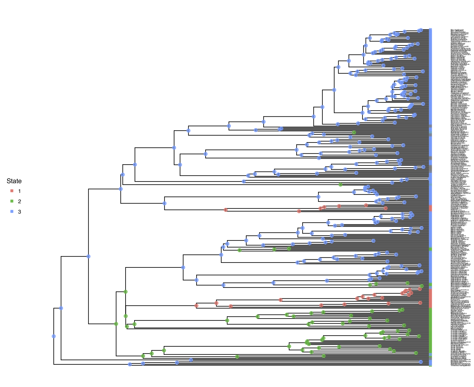
shows the result of this analysis.
Example: Unequal Transition Rates
Make a copy of the MCMC and model files you just made. Call them
mcmc_ase_mk.Revand `model_ase_FreeK.Rev. These will contain the new model parameters and models.
The Mk model makes a number of assumptions, but one that may strike you as unrealistic is the assumption that characters are equally likely to change from any one state to any other state. That means that a trait is as likely to be gained as lost. While this may hold true for some traits, we expect that it may be untrue for many others.
RevBayes has functionality to allow us to relax this assumption.
Modifying the MCMC Section
At each place in which the output files are specified in the MCMC file, change the output path so you don’t overwrite the output from the previous exercise.
For example, you might call your output file output/ase_freeK.log.
Change source statement to indicate the new model file.
Modifying the Model Section
Our goal here is to create a rate matrix with 6 free parameters. We will assume an exponential prior distribution for each of the rates. Thus, we start be specifying the rate of this exponential prior distribution. A good guess might be that 10 events happened along the tree, so the rate should be the tree-length divided by 10.
rate_pr := phylogeny.treeLength() / 10
Now we can create our six independent rate variables drawn from an identical exponential distribution
rate_12 ~ dnExponential(rate_pr)
rate_13 ~ dnExponential(rate_pr)
rate_21 ~ dnExponential(rate_pr)
rate_23 ~ dnExponential(rate_pr)
rate_31 ~ dnExponential(rate_pr)
rate_32 ~ dnExponential(rate_pr)
As usual, we will apply a scaling move to each of the rate variables.
moves.append( mvScale( rate_12, weight=2 ) )
moves.append( mvScale( rate_13, weight=2 ) )
moves.append( mvScale( rate_21, weight=2 ) )
moves.append( mvScale( rate_23, weight=2 ) )
moves.append( mvScale( rate_31, weight=2 ) )
moves.append( mvScale( rate_32, weight=2 ) )
Next, we put all the rates together into our rate matrix.
Don’t forget to say that we do not rescale the rate matrix (rescale=false).
We would only rescale if we use relative rates.
Q_morpho := fnFreeK( [ rate_12, rate_13, rate_21, rate_23, rate_31, rate_32 ], rescale=false )
In this model, we also decide to specify an additional parameter for the root state frequencies instead of assuming the root state to be drawn from the stationary distribution. We will use a Dirichlet prior distribution for the root state frequencies.
rf_prior <- [1,1,1]
rf ~ dnDirichlet( rf_prior )
moves.append( mvBetaSimplex( rf, weight=2 ) )
moves.append( mvDirichletSimplex( rf, weight=2 ) )
We need to modify the dnPhyloCTMC to pass in our new root frequencies parameter.
phyMorpho ~ dnPhyloCTMC(tree=phylogeny, Q=Q_morpho, rootFrequencies=rf, type="Standard")
Now you are done with your unequal rates model. Give it a run!
Reversible-jump MCMC to test for irreversibility
In the previous section we assumed that there are 6 different rates, which are all $>0$. Now, we will apply a reversible-jump MCMC (Green 1995) to test if any of the rates is significantly larger than $0$.
Make a copy of the Rev script file you just made. Call them `mcmc_ase_freeK_RJ.Rev. This will contain the new model parameters and models.
Modifying the MCMC Section
At each place in which the output files are specified in the MCMC section, change the output path so you don’t overwrite the output from the previous exercise.
For example, you might call your output file output/freeK_ASE.log.
Modifying the Model Section
The only part in the model section that we are going to modify is the prior distributions and moves on the rate parameters. We will assume the same rate for the exponential prior distribution as before.
rate_pr := phylogeny.treeLength() / 10
Next, we specify that we have a 0.5 probability, a priori, that a rate is equal to 0.
mix_pr <- 0.5
Now we can create our reversible-jump distributions, which take in a constant value, 0.0 in this case, and a distribution. Thus, the value is either drawn to be exactly equal to the constant value (0.0 here), or drawn from the base distribution (the exponential distribution in this case).
rate_12 ~ dnRJMixture(0.0, dnExponential(rate_pr), p=mix_pr)
rate_13 ~ dnRJMixture(0.0, dnExponential(rate_pr), p=mix_pr)
rate_21 ~ dnRJMixture(0.0, dnExponential(rate_pr), p=mix_pr)
rate_23 ~ dnRJMixture(0.0, dnExponential(rate_pr), p=mix_pr)
rate_31 ~ dnRJMixture(0.0, dnExponential(rate_pr), p=mix_pr)
rate_32 ~ dnRJMixture(0.0, dnExponential(rate_pr), p=mix_pr)
Since we are interested in the probability that a rate is equal to 0.0, we want to compute this posterior probability directly.
Therefore, we will use the ifelse function, which will return 1.0 if the rate is equal to 0.0, and 0.0 otherwise (if the rate is unequal to 0.0).
Hence, the frequency with which we sample a 1.0 gives us the posterior probability that a given rate is equal to 0.0.
prob_rate_12 := ifelse( rate_12 == 0, 1.0, 0.0 )
prob_rate_13 := ifelse( rate_13 == 0, 1.0, 0.0 )
prob_rate_21 := ifelse( rate_21 == 0, 1.0, 0.0 )
prob_rate_23 := ifelse( rate_23 == 0, 1.0, 0.0 )
prob_rate_31 := ifelse( rate_31 == 0, 1.0, 0.0 )
prob_rate_32 := ifelse( rate_32 == 0, 1.0, 0.0 )
We also need to specify specific moves that ``jump’’ in parameter dimension.
We will use the mvRJSwitch move that changes the value to be either equal to the constant value
provided from the dnRJMixture or a value drawn from the base distribution (the exponential distribution).
moves.append( mvRJSwitch( rate_12, weight=2 ) )
moves.append( mvRJSwitch( rate_13, weight=2 ) )
moves.append( mvRJSwitch( rate_21, weight=2 ) )
moves.append( mvRJSwitch( rate_23, weight=2 ) )
moves.append( mvRJSwitch( rate_31, weight=2 ) )
moves.append( mvRJSwitch( rate_32, weight=2 ) )
Additionally, we also need to specify moves that change the rates if they are not equal to 0.0. As usual, we use the standard scaling moves.
moves.append( mvScale( rate_12, weight=2 ) )
moves.append( mvScale( rate_13, weight=2 ) )
moves.append( mvScale( rate_21, weight=2 ) )
moves.append( mvScale( rate_23, weight=2 ) )
moves.append( mvScale( rate_31, weight=2 ) )
moves.append( mvScale( rate_32, weight=2 ) )
This is all that you need to do for this ``fancy’’ reversible-jump model. Give it a try!
Evaluate and Summarize Your Results
Visualizing Ancestral State Estimates
We have previously seen in how the ancestral states of the simple model look.
You should repeat plotting the ancestral states now also for the freeK and freeK_RJ analyses.
My output is shown in
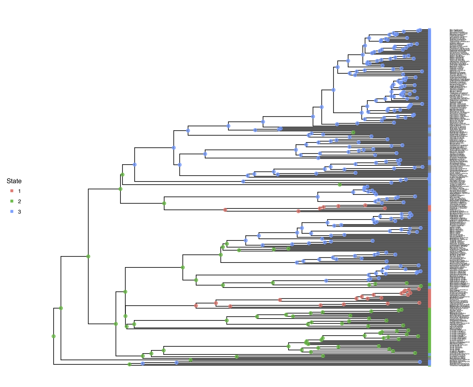
freeK model.You should observe that the estimated root states have changed!
- Green P.J. 1995. Reversible jump Markov chain Monte Carlo computation and Bayesian model determination. Biometrika. 82:711–732.
- Jukes T.H., Cantor C.R. 1969. Evolution of Protein Molecules. Mammalian Protein Metabolism. 3:21–132. 10.1016/B978-1-4832-3211-9.50009-7
- Lewis P.O. 2001. A Likelihood Approach to Estimating Phylogeny from Discrete Morphological Character Data. Systematic Biology. 50:913–925. 10.1080/106351501753462876
- PrabhuDas M., Bonney E., Caron K., Dey S., Erlebacher A., Fazleabas A., Fisher S., Golos T., Matzuk M., McCune J.M., others. 2015. Immune mechanisms at the maternal-fetal interface: perspectives and challenges. Nature immunology. 16:328–334.