Dating with Relative Constraints

Introduction

In phylogenetics, the term dating denotes the inference of node ages of phylogenies. For example, dating a species tree involves inference of the times when the species split. Dating phylogenies is central to understanding the evolution of life on Earth. However, evolutionary sequences evolve with different rates, an observation that has been termed relaxed molecular clock. In general, it is difficult to map a phylogeny obtained from a multiple sequence alignment, and with branch lengths measured in average number of substitutions per site, to a phylogeny with branch lengths measured in actual units of time. For this reason, the molecular clocks are calibrated with information gained from fossils, which can be accurately dated. Incorporating fossil information enables calibration of node ages of a phylogeny. Please also see the tutorial on fossil calibrations.

In this tutorial, we explore another possibility to improve on the accuracy of dating a phylogeny. Namely, horizontal gene transfers and ancient evolutionary relationships such as symbioses are informative about the order of nodes of a phylogeny of interest. That is, horizontal gene transfers define relative node constraints. Relative node constraints can be particularly helpful when the geological record is sparse, for example, for microorganisms, which represent the vast majority of extant and extinct biodiversity. Combination of node calibrations with relative node constraints can significantly improve both accuracy and resolution of molecular clock estimates (Szöllősi et al. 2021).

Definitions

Alignment: Multiple sequence alignment.

Timetree: Phylogeny with branch lengths measured in units of time. If the leaves have been sampled at the same time, for example, at the present, a time-tree is ultrametric.

Branch-length tree: Phylogeny with branch lengths measured in expected numbers of substitutions. Usually, branch-length trees are obtained from a phylogenetic analysis of an alignment.

Calibration: Absolute node calibration; an estimate of the age of a node of a timetree. This is usually associated with a prior describing the uncertainty associated to this node age.

Constraint: Relative node order constraint, which specifies the relative order in time of two nodes of a tree (e.g. node A is older than node B).

Getting Started

This tutorial was tested against the development branch, available at commit 06c1cac. Similar to other RevBayes tutorials, we suggest using the following directory structure:

.
├── data
├── scripts
└── output

The following data files are available:

data/
├── alignment.fasta    -- Alignment file simulated with the Jukes-Cantor (JC) model.
├── constraints.txt    -- File containing constraints.
├── substitution.tree  -- Tree with branch length in expected number of substitutions used to simulate the alignment.
└── time.tree          -- Original timetree to be recovered.

The following RevBayes script files are available:

scripts/
├── 1a_mcmc_jc.rev                   -- Infer branch-length trees using the JC model.
├── 1b_summarize_branch_lengths.rev  -- Extract posterior means and variances of branch lengths.
└── 2_mcmc_dating.rev                -- Date with calibrations and constraints.

Simulated data will be used, so that the inferred timetrees can be tested for accuracy against the correct timetree stored in the file time.tree. Inference will be done twice: (1) using calibrations only, and (2) using calibrations and constraints. We will not perform inference of the topology of the tree, only of the age of its nodes. We will therefore work with the correct, fixed tree topology obtained from the file substitution.tree. On empirical data, one could use the maximum-likelihood (ML) or the maximum a posteriori (MAP) topology obtained from a phylogenetic reconstruction based on the alignment as in e.g. tutorial Phylogenetic inference of nucleotide data using RevBayes.

Statement of the Problem

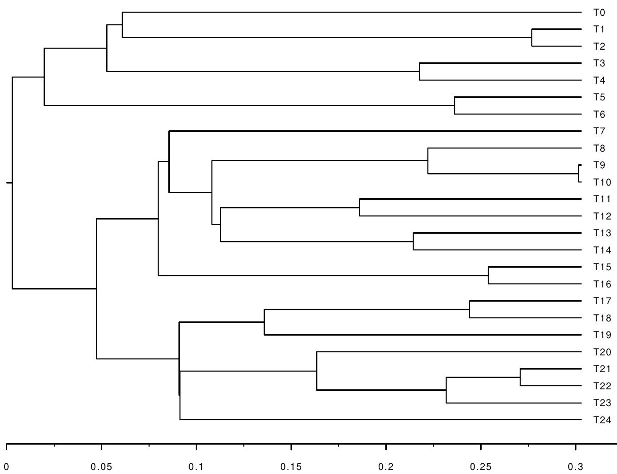
We are interested in inferring the following timetree using calibrations and constraints:

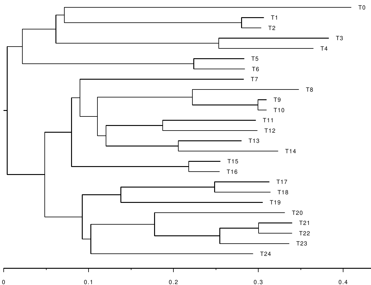
However, the only information we get is an alignment simulated along the following branch-length tree:

For reasons of computational efficiency, the phylogenetic likelihood is approximated using a branch-wise composition of normal distributions. For a detailed description of this two-step procedure please see (Szöllősi et al. 2021). In the first step, the posterior distributions of branch lengths for a fixed unrooted topology is inferred using the JC model (1a_mcmc_jc.rev). Then, the inferred posterior distributions of branch lengths are summarized into the posterior means and variances of the branch lengths (1b_summarize_branch_lengths.rev). In the second step, these posterior means and variances of the branch lengths, as well as the calibrations and constraints are used to date the phylogeny (2_mcmc_dating.rev).

The approximation of the phylogenetic likelihood using posterior means and variances is optional but recommended for reasons of computational efficiency. It is not necessary to use this approximation when dealing with relative time constraints, but the benefit here is clear: the first step computes branch-length tree distributions, which is costly and takes a long time. Once this has been done, in step two, several different dating models can be run efficiently without the need to rerun the analysis performed in the first step.

Step 1a: Inference of the Posterior Distributions of the Branch Lengths

Please execute the following command to perform Bayesian inference of the posterior distributions of branch-length trees using a Jukes-Cantor substitution model on a single alignment with a fixed tree topology. The Markov chain Monte Carlo (MCMC) algorithm runs for 30000 iterations. It uses the alignment data/alignment.fasta, and the branch-length tree data/substitution.tree. The output is a file output/alignment.fasta.trees containing the 30000 branch-length trees from the MCMC chain. It will be used to calculate the posterior means and variances of the branch lengths.

 rb ./scripts/1a_mcmc_jc.rev

For more detailed explanations of the script file, please consult the continuous time Markov chain tutorial.

Step 1b: Summarizing Branch Length Distributions by Means and Variances

In this step, we compute the means and variances of the posterior distributions of branch lengths using the 30000 trees obtained in step 1a. Please have a look at the script file scripts/1b_summarize_branch_lengths.rev.

First, we specify the name of the file containing the trees, and the amount of thinning we apply (thinning = 5 means that we take every fifth tree):

# File including trees obtained in step 1a.
tree_file="alignment.fasta.trees"
# Only use every nth tree to calculate the posterior means and variances.
thinning = 5

Then, the trees are loaded and thinned:

tre = readBranchLengthTrees(outdir+file_trees_only)

print("Number of trees before thinning: ")
print(tre.size())

# Perform thinning.
index = 1
for (i in 1:tre.size()) {
  if (i % thinning == 0) {
    trees[index] = tre[i]
    index = index + 1
  }
}

The posterior means and squared means (which will be used to calculate variances) are then computed:

print("Compute the posterior means and squared means of the branch lengths.")
num_branches = trees[1].nnodes()-1
bl_means <- rep(0.0,num_branches)
bl_squaredmeans <- rep(0.0,num_branches)

# Extract the posterior branch lengths. The index `i` is traversing the trees,
# the index `j` is traversing the branches.
for (i in 1:(trees.size())) {
  for (j in 1:num_branches ) {
    bl_means[j] <- bl_means[j] + trees[i].branchLength(j)
    bl_squaredmeans[j] <- bl_squaredmeans[j] + trees[i].branchLength(j)^2
    }
}

# Compute the posterior means and squared means.
for (j in 1:num_branches ) {
  bl_means[j] <- bl_means[j] / (trees.size())
  bl_squaredmeans[j] <- bl_squaredmeans[j] / (trees.size())
}

Finally, the posterior means and variances are stored in two trees having the same topology as the one used for inference. In this way we ensure that the posterior means and variances for the specific branches are tracked in a correct way.

The posterior variances are calculated using the standard formula \(Var(X) = E(X^2) - E(X)^2.\)

Here we save the posterior means in a separate tree so we can use them later.

print("Compute the tree with posterior means as branch lengths.")
meanTree = readBranchLengthTrees(outdir+file_trees_only)[1]

print("Original mean tree before changing branch lengths")
print(meanTree)

for (j in 1:num_branches ) {
  meanTree.setBranchLength(j, bl_means[j])
}

print("Tree with posterior means as branch lengths.")
print(meanTree)

writeNexus(outdir+tree_file+"_meanBL.nex", meanTree)
print("The tree with posterior mean branch lengths has been saved.")

We also save the posterior varainces in a separate tree so we can use them later.

print ("Compute tree with posterior variances as branch lengths.")
varTree = readBranchLengthTrees(outdir+file_trees_only)[1]

print("Original variance tree before changing branch lengths")
print(varTree)

# Here, the posterior variances are calculated using the well known formula
# Var(x) =E[X^2] - E[X]^2.
for (j in 1:num_branches ) {
  varTree.setBranchLength(j, abs ( bl_squaredmeans[j] - bl_means[j]^2) )
}

print("Tree with posterior variances as branch lengths.")
print(varTree)

writeNexus(outdir+tree_file+"_varBL.nex", varTree)
print("The tree with posterior variance branch lengths has been saved.")

To run the script, please execute

 rb ./scripts/1b_summarize_branch_lengths.rev

Step 2: Dating Using Calibrations and Constraints

Finally, we date the phylogeny using a relaxed clock model. Please have a look at the script 2_mcmc_dating.rev. Important parts will be explained in the following.

Options

First, let’s define some file names and options:

time_tree_file="data/time.tree"
constraints_file="data/constraints.txt"
mean_tree_file="output/alignment.fasta.trees_meanBL.nex"
var_tree_file="output/alignment.fasta.trees_varBL.nex"
out_bn="alignment.fasta.approx.dating"

# Show debug output?
debug = true
# Use relative constraints?
constrain = false
# Length of Markov chain.
mcmc_length = 50000
mcmc_burnin = 100
# The posterior branch length distribution of some branches of the first run has
# zero variance. In this case, set the variance to the following value.
var_min = 1e-6

Root Age

Then, the root age is calibrated using an interval around the true root age:

root_age <- tree.rootAge()
root_age_delta <- root_age / 5
root_age_min <- root_age - root_age_delta
root_age_max <- root_age + root_age_delta
root_time_real ~ dnUniform(root_age_min, root_age_max)
root_time_real.setValue(tree.rootAge())
root_time := abs( root_time_real )

The correct root age is obtained from the variable tree which was initialized to store the correct timetree. By doing this, we are benefiting from the fact that we know the true timetree. When analyzing an empirical data set for which the timetree is not known, one needs to find other ways to come up with a reasonable prior distribution for the root age. We set a uniform prior on the age of the root.

Setting up Constraints

If specified, we also load the constraints from the given file contraints.txt:

if (constrain) {
  out_bn = out_bn + "_cons"
  constraints <- readRelativeNodeAgeConstraints(file=constraints_file)
}

The file constraints.txt stores the constraints obtained from 3 hypothetical gene transfer events.

-- Contents of file `data/constraints.txt`
T0	T1	T14	T15
T7	T8	T19	T20
T3	T4	T8	T9

The first line T0\tT1\tT14\tT15 tells RevBayes that the most recent common ancestor (MRCA) of T0 and T1 has to be older than the MRCA of T14 and T15, and so on for the following lines. You can look for the respective nodes on the timetree given above, and check that the constraints are actually valid. In fact, the constraints may be helpful in that they resolve the order of nodes having similar ages.

Yule Tree Model

Next, we use a birth process with an unknown birth rate as a prior for the timetree psi, and define some proposals for the MCMC sampler. The proposals change the root age, scale the branches of psi, and slide the nodes.

################################################################################
# Tree model.

birth_rate ~ dnExp(1)
moves.append(mvScale(birth_rate, lambda=1.0, tune=true, weight=3.0))

if (!constrain) psi ~ dnBDP(lambda=birth_rate, mu=0.0, rho=1.0, rootAge=root_time, samplingStrategy="uniform", condition="survival", taxa=taxa)
if (constrain) psi ~  dnConstrainedNodeOrder(dnBDP(lambda=birth_rate, mu=0.0, rho=1.0, rootAge=root_time, samplingStrategy="uniform", condition="survival", taxa=taxa), constraints)

psi.setValue(tree)
if (debug == true) {
  print("The original time tree:")
  print(tree)
  print("The tree used in the Markov chain:")
  print(psi)
}

moves.append(mvScale(root_time_real, weight=1.0, lambda=0.1))
moves.append(mvSubtreeScale(psi, weight=1.0*n_branches))
moves.append(mvNodeTimeSlideUniform(psi, weight=1.0*n_branches))
moves.append(mvLayeredScaleProposal(tree=psi, lambda=0.1, tune=true, weight=1.0*n_branches))

Adding Node Calibrations

Now, two calibrations are added. The MRCAs of T1 and T2, as well as T14 and T15 are fixed to be within intervals centered around their true ages (initially, psi stores the true tree). The distribution dnSoftBoundUniformNormal is uniform between the specified boundaries and decreases normally out of the boundaries with the given standard deviation (sd).

################################################################################
# Node calibrations provide information about the ages of the MRCA.

# The MRCAs of the following clades are calibrated.
clade_0 = clade("T1","T2")
clade_1 = clade("T14","T15")

# Clade 0.
tmrca_clade_0 := tmrca(psi, clade_0)
age_clade_0_mean <- tmrca(psi, clade_0)
age_clade_0_delta <- age_clade_0_mean / 5
age_clade_0_prior ~ dnSoftBoundUniformNormal(min=age_clade_0_mean-age_clade_0_delta, max=age_clade_0_mean+age_clade_0_delta, sd=2.5, p=0.95)
age_clade_0_prior.clamp(age_clade_0_mean)

# Clade 1.
tmrca_clade_1 := tmrca(psi, clade_1)
age_clade_1_mean <- tmrca(psi, clade_1)
age_clade_1_delta <- age_clade_1_mean / 5
age_clade_1_prior ~ dnSoftBoundUniformNormal(min=age_clade_1_mean-age_clade_1_delta, max=age_clade_1_mean+age_clade_1_delta, sd=2.5, p=0.95)
age_clade_1_prior.clamp(age_clade_1_mean)

Posterior Means and Variances

Finally, we read in the posterior means and variances of the branch lengths prepared in the step 1b.

mean_tree <- readTrees(mean_tree_file)[1]
var_tree <- readTrees(var_tree_file)[1]

We re-root the timetrees and ensure that they are bifurcating. These steps are necessary to get the correct mapping between branches, and their posterior means and variances. Internally, it is ensured that the indices are shared correctly.

# Reroot and make bifurcating.
rootId <- tree.getRootIndex()
outgroup <- tree.getDescendantTaxa(rootId)
mean_tree.reroot(clade=clade(outgroup), make_bifurcating=TRUE)
var_tree.reroot(clade=clade(outgroup), make_bifurcating=TRUE)

# Renumber nodes.
mean_tree.renumberNodes(tree)
var_tree.renumberNodes(tree)

Further, this step harbors a complication. During the first step, the reversible JC model was used to estimate the posterior means and variances of the branch lengths. Hence, the estimated branch-length tree is unrooted. Now, we estimate a rooted time tree. It follows that the two branches leading to the root of the timetree correspond to a single branch of the unrooted tree from the first step. We have to take this into account when approximating the phylogenetic likelihood.

# Get indices of left child and right child of root.
i_left <- tree.child(tree.nnodes(),1)
i_right <- tree.child(tree.nnodes(),2)

# Get posterior means and variances of all branches except the branches leading
# to the root.
for(i in 1:n_branches) {
  if(i != i_left && i != i_right) {
    posterior_mean_bl[i] <- mean_tree.branchLength(i)
    posterior_var_bl[i] := var_tree.branchLength(i)
    if (posterior_var_bl[i]<var_min) posterior_var_bl[i]:=var_min
  }
}

# Get the index of the root in the time tree.
if (i_left<i_right)  i_root <- i_left
if (i_left>=i_right) i_root <- i_right

# Get the mean and variance of the branch containing the root.
posterior_mean_bl_root <- mean_tree.branchLength(i_root)
posterior_var_bl_root <- var_tree.branchLength(i_root)
if (posterior_var_bl_root<var_min) posterior_var_bl_root:=var_min

Please also note that we set a minimum variance. In some extreme cases, the posterior distribution of a branch length may be so condensed, that the variance is too low to be used for calculating the approximate phylogenetic likelihood.

Relaxed Molecular Clock Model

In the next step, we define the relaxed molecular clock model. Several of them are available in RevBayes. Here, we decided to use an uncorrelated model. We separate between a global rate (global_rate_mean) and the relative branch-wise rates (rel_branch_rates). We use an uncorrelated gamma model (UGAM). In the UGAM model, the relative branch rates are distributed according to a gamma distribution. We use a hyper parameter sigma on the shape and scale parameters of the gamma distribution:

mean_tree_root_age := mean_tree.rootAge()
global_rate_mean ~ dnExp(1)
global_rate_mean.setValue(mean_tree_root_age/tree.rootAge());
sigma ~ dnExp(10.0)

first_gamma_param := 1/sigma
second_gamma_param := 1/sigma

moves.append(mvScaleBactrian(global_rate_mean, lambda=0.5, weight=10.0))
moves.append(mvScaleBactrian(sigma, lambda=0.5, weight=10.0))

# Use a Gamma distribution on rates.
for (i in n_branches:1) {
  times[i]=psi.branchLength(i)
  rel_branch_rates[i] ~ dnGamma(first_gamma_param, second_gamma_param)
  # Exclude the branches leading to the root (see above).
  if(i != i_left && i != i_right) {
    rel_branch_rates[i].setValue(posterior_mean_bl[i]/times[i]/global_rate_mean)
  } else {
    # And set them to half of the branch length in the unrooted tree.
    rel_branch_rates[i].setValue(posterior_mean_bl_root/2/times[i]/global_rate_mean)
  }
  moves.append(mvScale(rel_branch_rates[i], lambda=0.5, weight=1.0,tune=true))
}

for (i in n_branches:1) {
  branch_rates[i] := global_rate_mean * rel_branch_rates[i]
}

Likelihood

Finally, we calculate the approximate phylogenetic likelihood. In detail, for each branch, the length measured in substitutions is the product of the length measured in time, and the evolutionary rate at that branch:

mean_bl[i] := times[i]*branch_rates[i]

The branch lengths are then distributed according to normal distributions with the posterior means and variances obtained in the previous step:

bls[i] ~ dnNormal(mean_bl[i] ,sqrt(posterior_var_bl[i]))

Again, the two branches leading to the root are handled in a special way. In total, the approximate phylogenetic likelihood is calculated like so:

times[i_left] := psi.branchLength(i_left)
times[i_right] := psi.branchLength(i_right)

for(i in 1:n_branches) {
  if(i != i_left && i != i_right) {
    times[i] := psi.branchLength(i)
    mean_bl[i] := times[i]*branch_rates[i]
    bls[i] ~ dnNormal(mean_bl[i] ,sqrt(posterior_var_bl[i]))
    bls[i].clamp(posterior_mean_bl[i])
  }
}

# See above.
mean_bl_root := times[i_left]*branch_rates[i_left] + times[i_right]*branch_rates[i_right]
bls[i_root] ~ dnNormal(mean_bl_root, sqrt(posterior_var_bl_root))
bls[i_root].clamp(posterior_mean_bl_root)

Monitors and MCMC

The last part of the script defines the monitors, executes the MCMC chain, and saves the results.

Define the monitors:

for(i in 1:n_branches)
{
  ages_psi[i] := psi.nodeAge(i)
  ages_true[i] := tree.nodeAge(i)
}
if (debug == true) {
  print("True node ages:")
  print(ages_true)
  print("Node ages of state of Markov chain:")
  print(ages_psi)
}

trees_base_name = "output/" + out_bn
trees_file_name = trees_base_name + ".trees"
monitors.append(mnModel(filename="output/"+out_bn+".log",printgen=10, separator = TAB))
monitors.append(mnStochasticVariable(filename="output/"+out_bn+"_Stoch.log",printgen=10))
monitors.append(mnExtNewick(filename=trees_file_name, isNodeParameter=FALSE, printgen=10, separator = TAB, tree=psi, branch_rates))

# Add some random age monitors.
monitors.append(mnScreen(printgen=100, root_time, ages_psi[20], ages_psi[25], ages_psi[27]))

Use the Metropolis-coupled Markov chain Monte Carlo algorithm:

# mymodel = model(branch_rates)
mymodel = model(bls)
mymcmc = mcmcmc(mymodel, monitors, moves, nruns=1, nchains=4, tuneHeat=TRUE)
mymcmc.burnin(generations=mcmc_burnin,tuningInterval=mcmc_burnin/10)
mymcmc.operatorSummary()
mymcmc.run(generations=mcmc_length)
mymcmc.operatorSummary()

To perform the dating analysis, please execute twice (once with constrain = true, and once with constrain = false):

rb ./scripts/2_mcmc_dating.rev

The MAP trees for the analysis with calibrations only, and with calibrations and constraints are stored in the files output/alignment.fasta.approx.dating.tree, and output/alignment.fasta.approx.dating_cons.tree, respectively.

Analysis of results

The following figures show the inferred timetrees.

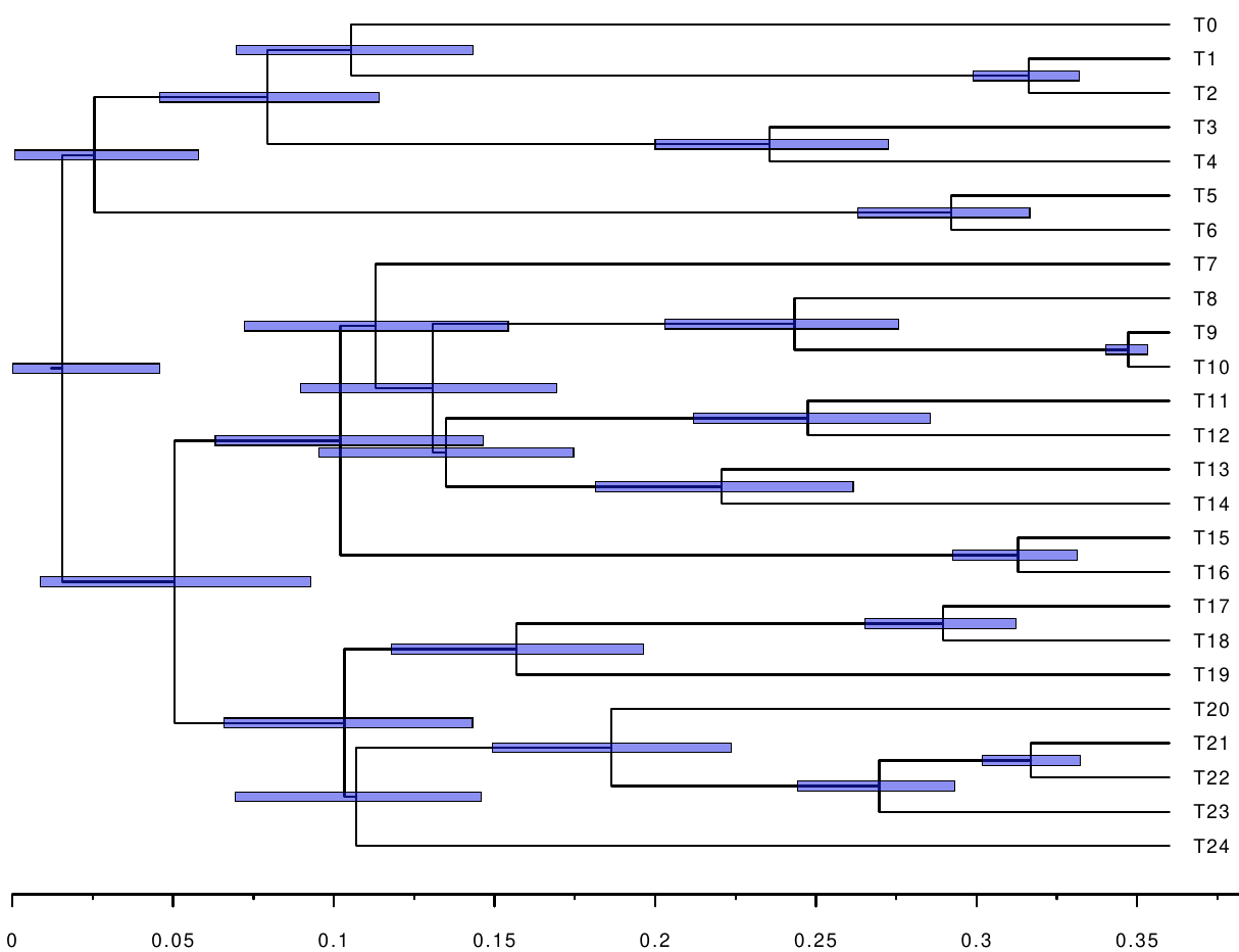
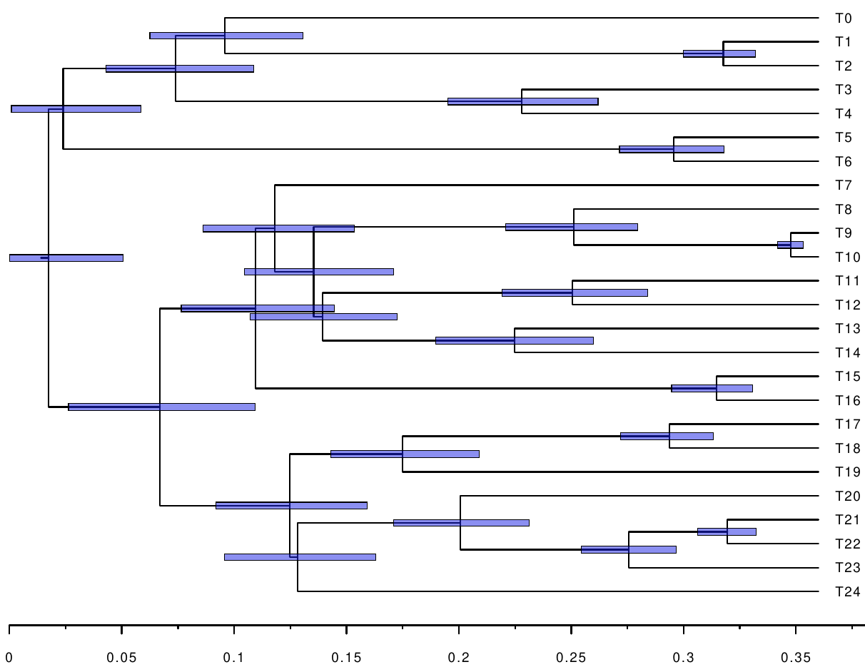
We see that the constraints help improve the accuracy, as well as reduce the confidence intervals of the node ages. Further, we can measure the distance between the inferred timetrees, and the original timetree used for simulating the alignment. We use the branch score distance

where $T_1$ and $T_2$ are two trees, $i$ traverses the branches, and $\Delta_i$ is the difference of the lengths of the branch in $T_1$ and $T_2$. If a branch is only in one tree, the whole length is chosen (although this is not the case here). The branch score distances can be calculated with any phylogenetic software package. Here, we used ELynx. The branch score distances between the original timetree, and the inferred timetrees are:

$ tlynx distance -d branch-score -f RevBayes -m data/time.tree output/alignment.fasta.approx.dating.tree output/alignment.fasta.approx.dating_cons.tree
=== tlynx
Compare, examine, and simulate phylogenetic trees.
ELynx Suite version 0.4.0.
Developed by Dominik Schrempf.
Compiled on September 19, 2020, at 13:41 pm, UTC.
Start time: October 9, 2020, at 11:29 am, UTC.
Command line: tlynx distance -d branch-score -f RevBayes -m data/time.tree output/alignment.fasta.approx.dating.tree output/alignment.fasta.approx.dating_cons.tree

Write results to standard output.
Read master tree from file: data/time.tree.
Compute distances between all trees and master tree.
Read trees from files.
Trees are named according to their file names.
Use branch score distance.
Summary statistics of Branch Score Distance:
Mean:     0.151
Median:   0.159
Variance: 0.000

Tree 1                                          Tree 2                                            Branch Score
data/time.tree                                  output/alignment.fasta.approx.dating.tree                0.159
data/time.tree                                  output/alignment.fasta.approx.dating_cons.tree           0.142
No output file given --- skip writing ELynx file for reproducible runs.
=== End time: October 9, 2020, at 11:29 am, UTC.

That is, using constraints helped improve the branch score distance by 11 percent.

Concluding remarks

When analyzing real data a more appropriate substitution model should be used. Also, when the tree topology is unknown, it has to be inferred. This has to be done beforehand. Finally, calibrations and constraints have to be obtained manually either based on the literature or based on original research.

The simulations were done using a custom simulator called ELynx. If you are interested, please have a look at the source code of ELynx and the simulation scripts for this tutorial.

1. Szöllősi G.J., Höhna S., Williams T.A., Schrempf D., Daubin V., Boussau B. 2021. Relative time constraints improve molecular dating. Manuscript in preparation.