Introduction
In the Simple phylogenetic analysis using the DEC model tutorial, we went through the exercise of setting up the instantaneous rate matrix and cladogenetic transition probabilities for a simple DEC model. In this tutorial, we will set up a more complex model considering the geological histories in the biogeographic inference. We will learn how to set up an epoch model.
An improved DEC analysis
In this section, we’ll introduce a suite of model features that lend towards more realistic biogeographic analyses. Topics include applying range size constraints, stratified (or epoch) models of paleoconnectivity, function-valued dispersal rates, and incorporating uncertainty in paleogeographic event time estimates. These modifications should produce more realistic ancestral range estimates, e.g. that a volcanic island may only be colonized once it has formed, and that distance should have some bearing on dispersal rate.
To accomplish this, we’ll incorporate (paleo-)geographical data for the Hawaiian archipelago, summarized in . Even though we will continue to use four areas (K, O, M, H) in this section, we will use all six areas (R, K, O, M, H, Z) in , hence the full table is given for future reference.
| area | code | $a_{max}$ | $a_{min}$ | $g_{\bullet R}$ | $g_{\bullet K}$ | $g_{\bullet O}$ | $g_{\bullet M}$ | $g_{\bullet H}$ | $g_{\bullet Z}$ |
|---|---|---|---|---|---|---|---|---|---|
| Older islands | R | - | - | - | 261 | 406 | 500 | 680 | 3900 |
| Kauai | K | 5.15 | 5.05 | - | - | 145 | 239 | 419 | 3900 |
| Oahu | O | 3.7 | 2.2 | - | - | - | 059 | 239 | 3900 |
| Maui Nui | M | 1.8 | 1.3 | - | - | - | - | 082 | 3900 |
| Hawaii | H | 0.7 | 0.3 | - | - | - | - | - | 3900 |
| Mainland | Z | - | - | - | - | - | - | - | - |
Analysis
Start by creating variables for the tree file, the range data, and the output prefix
    range_fn = "data/n4/silversword.n4.range.nex"
    tree_fn = "data/n4/silversword.tre"
    out_fn = "output/epoch"
The paleogeographical information from is encoded
in three files named hawaii.n4.times.txt,
hawaii.n4.distances.txt, and
hawaii.n4.connectivity.*.txt.
    geo_fn = "data/n4/hawaii.n4"
    times_fn = geo_fn + ".times.txt"
    dist_fn = geo_fn + ".distances.txt"
Create vectors that will contain all of our moves and monitors vectors, respectively.
    moves = VectorMoves()
    monitors = VectorMonitors()
Read in the presence-absence range characters and record the number of areas in the dataset
    dat_range_01 = readDiscreteCharacterData(range_fn)
    n_areas <- dat_range_01.nchar()
Often, biogeographers wish to limit to the maximum allowable range size. This prohibits widespread species ranges and reduces the total number of range states in the analysis, thus improving computational efficiency. We will restrict ranges from including more than two areas. The total number of ranges equals $\sum_{k=0}^m {n \choose k}$ where $n$ is the total number of areas, $m$ is the maximum number of permissible areas, and ${n}\choose{k}$ is the number of ways to sample $k$ unordered areas from a pool of $n$ areas. For $n=4$ and $m=2$, this equals ${4 \choose 0} + {4 \choose 1} + {4 \choose 2} = 1 + 4 + 6 = 11$ states.
First, compute the number of states
    max_areas <- 2
    n_states <- 0
    for (k in 0:max_areas) n_states += choose(n_areas, k)
then use n_states to format the dataset for the reduced state space
dat_range_n = formatDiscreteCharacterData(dat_range_01, "DEC", n_states)
Our state space now includes only 11 states ($\emptyset$, K, O, M, H, KO, KM, OM, KH, OH, MH).
Record the complete list of range descriptions to file
    state_desc = dat_range_n.getStateDescriptions()
    state_desc_str = "state,range\n"
    for (i in 1:state_desc.size())
    {
        state_desc_str += (i-1) + "," + state_desc[i] + "\n"
    }
    write(state_desc_str, file=out_fn+".state_labels.txt")
As with the previous analysis, we’ll brazenly assume we know the dated species phylogeny without error.
tree <- readTrees(tree_fn)[1]
Next, we’ll read and structure our paleogeographic data. Read in the list of minimum and maximum ages of island formation
    time_bounds <- readDataDelimitedFile(file=times_fn, delimiter=" ")
    n_epochs <- time_bounds.size()
Read in the vector of matrices that describe the connectivity between areas over time. Note, there is one connectivity matrix per epoch, ordered from oldest to youngest.
    for (i in 1:n_epochs) {
      epoch_fn[i] = geo_fn + ".connectivity." + i + ".txt"
      connectivity[i] <- readDataDelimitedFile(file=epoch_fn[i], delimiter=" ")
    }
The area connectivity file for the third epoch (when K, O, and M exist, but not H) contains
    1 1 1 0
    1 1 1 0
    1 1 1 0
    0 0 0 0
Dispersal events between, say, K and M will be penalized by distance rather than be forbidden by non-connectivity.
Read in the matrix of distances between all pairs of areas (km). For simplicity, we will assume that distances remained constant across epochs, even though these distances certainly varied over time.
distances <- readDataDelimitedFile(file=dist_fn, delimiter=" ")
The distances files contains
    001 145 239 419
    145 001 059 239
    239 059 001 082
    419 239 082 001
and, if we assume the relative distance between islands remains roughly constant over time, then one set of distances is suitable for use for all four epochs.
Next, we’ll build an enhanced DEC model. Like before, we’ll define the
rate matrix in terms of relative rates, then rescale the entire matrix
with the biogeographic rate scaling parameter rate_bg.
    rate_bg ~ dnLoguniform(1E-4,1E2)
    rate_bg.setValue(1E-2)
And create a move to update the base rate of anagenetic change
moves.append( mvSlide(rate_bg, weight=4) )
Fix the base dispersal rate to 1
dispersal_rate <- 1.0
Dispersal rates might make use of some extrinsic information, such as geographical distances between areas (MacArthur and Wilson 1967; Webb and Ree 2012). We model this as $d_{ij} = \exp(-a g_{ij})$ where $g_{ij}$ is the geographical distance between areas $i$ and $j$ and $a$ is a parameter that scales distance. Note that all dispersal rates are equal when $a=0$. Add a distance scale parameter
    distance_scale ~ dnUnif(0,20)
    distance_scale.setValue(0.01)
    moves.append( mvScale(distance_scale, weight=3) )
Now we can assign rates that are functions of distance between all pairs
of areas, but also over all epochs. To accomplish this,
notice we now have an outer loop over the number of epochs,
n_epochs. This is used to construct a vector of dispersal
matrices, one matrix per epoch. It is crucial to note that all of
elements are assigned the value 0.0 unless the if-statement
if (connectivity[i][j][k] > 0) evaluates to
true. That is, dispersal rates between areas j
and k for epoch i are non-zero if and only if
the connectivity matrix element connectivity[i][j][k]
has a positive value! When this condition is met, the dispersal rate is
determined by the exponential function of inverse distance given above.
    for (i in 1:n_epochs) {
      for (j in 1:n_areas) {
        for (k in 1:n_areas) {
          dr[i][j][k] <- 0.0
          if (connectivity[i][j][k] > 0) {
            dr[i][j][k]  := dispersal_rate * exp(-distance_scale * distances[j][k])
          }
        }
      }
    }
We will assign the same extirpation prior as was done in the simple analysis in the previous section
    log_sd <- 0.5
    log_mean <- ln(1) - 0.5*log_sd^2
    extirpation_rate ~ dnLognormal(mean=log_mean, sd=log_sd)
    moves.append( mvScale(extirpation_rate, weight=2) )
and then provide the appropriate extirpation matrix structure
    for (i in 1:n_epochs) {
      for (j in 1:n_areas) {
        for (k in 1:n_areas) {
          er[i][j][k] <- 0.0
        }
        er[i][j][j] := extirpation_rate
      }
    }
Now we have a vector of dispersal rates, dr, and an vector
of extirpation rates, er, in stored in the RevBayes
workspace. We’ll use these to create a vector of four DEC rate matrices,
one for each epoch.
    for (i in 1:n_epochs) {
      Q_DEC[i] := fnDECRateMatrix(dispersalRates=dr[i],
                                  extirpationRates=er[i],
                                  maxRangeSize=max_areas)
    }
Next, we need to define breakpoints for when the underlying paleogeographic state/connectivity changes. In our case, we’ll define the epoch breakpoints as uniformly distributed random variables that are bounded by the minimum and maximum age estimates for when each new island complex formed (). This is easily done using a for loop over the number of epochs. Note, we define the end of the final epoch as the present.
    for (i in 1:n_epochs) {
      time_max[i] <- time_bounds[i][1]
      time_min[i] <- time_bounds[i][2]
      if (i != n_epochs) {
          epoch_times[i] ~ dnUniform(time_min[i], time_max[i])
          moves.append( mvSlide(epoch_times[i], delta=(time_max[i]-time_min[i])/2) )
      } else {
          epoch_times[i] <- 0.0
      }
    }
Now that we have variables for the timing (epoch_times)
and character (Q_DEC via connectivity) of
paleogeographic change throughout the Hawaiian archipelago, we’re ready
to unify these objects with the fnEpoch function. This
function requires a vector of rate matrices, a vector of epoch end
times, and a vector of rate multipliers as arguments. Internally, the
function computes the appropriate probabilities for state transitions
along branches according under a piecewise constant continuous-time
Markov chain. The important consequence of using an epoch model is that
transition probabilities for anagenetic events depend on the geological
age of the branch.
Q_DEC_epoch := fnEpoch(Q=Q_DEC, times=epoch_times, rates=rep(1,n_epochs))
Here, we treat the probability of different types of cladogenetic events as a random variables to be estimated.
    clado_event_types <- [ "s", "a" ]
    p_sympatry ~ dnUniform(0,1)
    p_allopatry := abs(1.0 - p_sympatry)
    clado_type_probs := simplex(p_sympatry, p_allopatry)
    moves.append( mvSlide(p_sympatry, weight=2) )
    P_DEC := fnDECCladoProbs(eventProbs=clado_type_probs,
                             eventTypes=clado_event_types,
                             numCharacters=n_areas,
                             maxRangeSize=max_areas)
For this dataset, we assume cladogenetic probabilities are constant with
respect to geological time. Using time-dependent cladogenetic
probabilities (fnEpochCladoProbs) and mixtures of
cladogenetic probabilities (fnMixtureCladoProbs) will be
covered in future tutorials.
Among the four areas, only Kauai existed at the provided origination time of the clade, so will set it as the only valid starting state through the root frequency distribution.
    rf_DEC_tmp <- rep(0, n_states)
    rf_DEC_tmp[2] <- 1
    rf_DEC <- simplex(rf_DEC_tmp)
We have created all the necessary model variables. Now we can create the
phylogenetic model of anagenetic and cladogenetic character evolution.
dnPhyloCTMCClado will internally make use of the
time-heterogeneous probabilities embedded in the epoch rate generator,
Q_DEC_epoch.
    m_bg ~ dnPhyloCTMCClado(tree=tree,
                            Q=Q_DEC_epoch,
                            cladoProbs=P_DEC,
                            branchRates=rate_bg,
                            rootFrequencies=rf_DEC,
                            type="NaturalNumbers",
                            nSites=1)
Attach the observed range data to the distribution
m_bg.clamp(dat_range_n)
And the rest we’ve done before…
    monitors.append( mnScreen(printgen=100, rate_bg, extirpation_rate, distance_scale) )
    monitors.append( mnModel(file=out_fn+".model.log", printgen=10) )
    monitors.append( mnFile(tree, filename=out_fn+".tre", printgen=10) )
    monitors.append( mnJointConditionalAncestralState(tree=tree,
                                                           ctmc=m_bg,
                                                           type="NaturalNumbers",
                                                           withTips=true,
                                                           withStartStates=true,
                                                           filename=out_fn+".states.log",
                                                           printgen=10) )
    monitors.append( mnStochasticCharacterMap(ctmc=m_bg,
                                              filename=out_fn+".stoch.log",
                                              printgen=100) )
Wrap the model graph into a model object
mymodel = model(m_bg)
then build and run MCMC
    mymcmc = mcmc(mymodel, moves, monitors)
    mymcmc.run(5000)
Results
Example results are located at output_example/epoch.
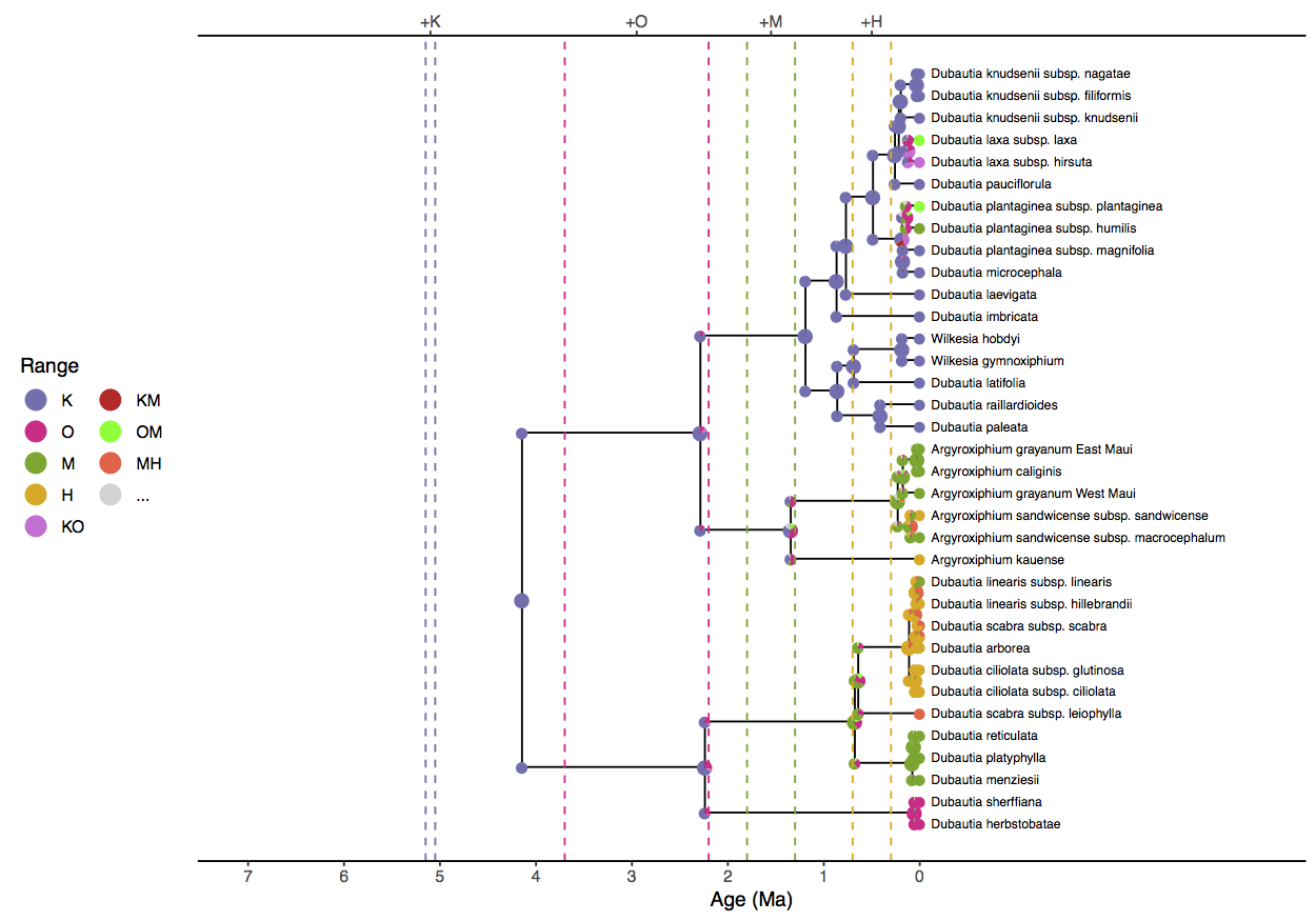
When compared to the ancestral state estimates from the “simple” analysis (Simple phylogenetic analysis using the DEC model), these results are far more consonant with what we understand about the origination times of the islands (). First, this reconstruction asserts that the clade originated in the modern Hawaiian islands at a time when only Kauai was above sea level. Similarly, the D. sheriffiana and D. arborea clade no longer estimates OMH as its ancestral range, since Maui and Hawaii had not yet formed 2.4 Ma. The ancestral range for the Agyroxiphium clade does not have a Hawaiian origin, whereas previously it awarded substantial support for H or MH origins.
It may be that these epoch-based estimates are relatively accurate, or they may contain artifacts as a result of assuming a fixed and errorless phylogeny. The next tutorials discuss how to jointly estimate phylogeny and biogeography, which potentially improves the estimation of divergence times, tree topology, and ancestral ranges.
Continue to the next tutorial: Biogeographic dating using the DEC model
- Landis M.J., Freyman W.A., Baldwin B.G. 2018. Retracing the Hawaiian silversword radiation despite phylogenetic, biogeographic, and paleogeographic uncertainty. Evolution. 72:2343–2359.
- Lim J.Y., Marshall C.R. 2017. The true tempo of evolutionary radiation and decline revealed on the Hawaiian archipelago. Nature. 543:710–713.
- MacArthur R.H., Wilson E.O. 1967. Theory of Island Biogeography. Princeton University Press. 10.1515/9781400881376
- Webb C.O., Ree R.H. 2012. Historical biogeography inference in Malesia. Biotic evolution and environmental change in Southeast Asia.:191–215. 10.1017/CBO9780511735882.010