Discrete morphology - Correlation among Characters

Overview

In this tutorial we want to test for correlation between two discrete characters. In this primates dataset, we have the following discrete morpholigical characters: activity period, habitat, solitariness, terrestrially, number of males per group, mating system and diet (see Introduction to Discrete Morphology Evolution for more details). For example, the habitat and terrestrially characters are very likely to be dependent on another. But what about the other characters and how do we test for correlation? It actually turns out to be very similar to our Discrete morphology - Stochastic Character Mapping and Hidden Rates analysis.

The Correlated Evolution Model

In this exercise, let us assume that we have two binary characters A and B. To test for correlation, we need to combine these two characters into a single one. That means, we will expand the state space to 00, 10, 01 and 11 where the first position corresponds to the state of character A and the second position corresponds to character B. If both characters evolve independently and according to rates of gain $\alpha_A$ and $\alpha_B$ and rates of loss $\beta_A$ and $\beta_B$, respectively, then we can write the rate matrix as follows (Pagel and Meade 2004).

Now if we assume instead that rates of gain and loss for both characters actually depend on the state of the other character, then we would obtain the full rate matrix of

Note that only single transitions, i.e., a transition of one character and not both, are allowed at a time. That is, we assume that not both characters can be gained or lost at the same infinitesimal small time interval, and instead that one usually precedes the other.

In the first rate matrix, we only had 4 parameters. Now in the second rate matrix, we have 8 parameters. If we want to test for correlations, we can simply test if specific parameters are indeed distinguishable (Pagel and Meade 2004).

These parameters are:

• $\mu_{1,2} \neq \mu_{3,4}$: a gain in character A does not depend on the state of character B
• $\mu_{2,1} \neq \mu_{4,3}$: a loss in character A does not depend on the state of character B
• $\mu_{1,3} \neq \mu_{2,4}$: a gain in character B does not depend on the state of character A
• $\mu_{3,1} \neq \mu_{4,2}$: a loss in character B does not depend on the state of character A

We will perform these tests here using reversible jump Markov chain Monte Carlo.

Let us start with a fresh Rev script. Create an empty text file and call it `mcmc_corr_RJ.Rev.

Load the Data Matrices

As before, use the function readDiscreteCharacterData() to load a data matrix to the workspace from a formatted file. However, this time we need to load two data matrices, one for each character.

morpho_A <- readDiscreteCharacterData("data/primates_solitariness.nex")
morpho_B <- readDiscreteCharacterData("data/primates_terrestrially.nex")

Next, we need to combine the 2 character into a single one. In RevBayes, there is a convenient way so you don’t have to do it manually. You can use the function combineCharacter() which will combine any two characters.

morpho = combineCharacter( morpho_A, morpho_B )

Again, to get a better understanding of how this happened just look into the newly created character data matrix (and the original ones if you want too).

morpho

   NaturalNumbers character matrix with 233 taxa and 1 characters
   ==============================================================
   Origination:                   
   Number of taxa:                233
   Number of included taxa:       233
   Number of characters:          1
   Number of included characters: 1
   Datatype:                      NaturalNumbers

Notice that the Datatype for this character data matrix is NaturalNumbers. In RevBayes, we always default back to NaturalNumbers as the data type because we can list arbitrarily many states, but for standard states we wouldn’t know how to label them (except going through the alphabet, which is clearly shorter and doesn’t have any more meaning than numbers).

Let us now also look at how the states are combined. Again, we look first at the original character data matrix.

morpho.show()

   Allenopithecus_nigroviridis
   1
   Allocebus_trichotis
   2
   Alouatta_belzebul
   0
   Alouatta_caraya
   0
   Alouatta_coibensis
   0
   Alouatta_fusca
   0
   Alouatta_palliata
   0
   Alouatta_pigra
   0
   Alouatta_sara
   (0 2)
   Alouatta_seniculus
   0
   Aotus_azarai
   0
   Aotus_brumbacki
   (0 2)
   Aotus_hershkovitzi
   (0 2)
   ...

We see that Allenopithecus nigroviridis has state 1 and Allocebus trichotis has state 2. There are also ambiguous states if one or both character were ambiguous or missing. It is important to remember how the state space was expanded to set the rates up correctly.

Create Helper Variables

As before, we need to instantiate a couple “helper variables” that will be used by downstream parts of our model specification files. Create vectors of moves and monitors

moves = VectorMoves()
monitors = VectorMonitors()

The Phylogeny

As usual for morphological analysis, we assume the phylogeny to be know. Thus, we read in the tree as a constant variable:

phylogeny <- readTrees("data/primates_tree.nex")[1]

The Correlated Rates Model

Now we need to specify the correlated rates model. Have a look again above at the rate matrix that we want to specify. In the current example, we assume two binary morphological character. This gives 4 states in total and therefore a 4x4 rate matrix.

Start with creating a matrix called rates where all elements are 0.0.

# we will fill the non-zero elements below
for (i in 1:4) {
  for (j in 1:4) {
    rates[i][j] <- 0.0
  }
}

Next, we specify the global rate prior. As in all previous discrete morphological evolution excersises, we will use an exponential prior distribution with a mean of 10 events along the given phylogeny.

rate_pr := phylogeny.treeLength() / 10

We also specify a prior probability of 0.5 that each pair of rates is indeed correlated.

mix_prob <- 0.5

Then, let us specify the rate of gain for character A. First, we do this for the case when character B is in state 0. We will assume an exponential prior distribution here.

rate_gain_A_when_B0 ~ dnExponential( rate_pr )

Second, we create the rate for a gain in character A when character B is in state 1. This can either be the same rate (i.e., independent of the state of B) or its own rate. Therefore we use the reversible jump mixture distribution.

rate_gain_A_when_B1 ~ dnReversibleJumpMixture(rate_gain_A_when_B0, dnExponential( rate_pr ), mix_prob)

Now proceed in the same way for the rate of loss in character A, the rate of gain in character B and the rate of loss in character B.

rate_loss_A_when_B0 ~ dnExponential( rate_pr )
rate_loss_A_when_B1 ~ dnReversibleJumpMixture(rate_loss_A_when_B0, dnExponential( rate_pr ), mix_prob)

rate_gain_B_when_A0 ~ dnExponential( rate_pr )
rate_gain_B_when_A1 ~ dnReversibleJumpMixture(rate_gain_B_when_A0, dnExponential( rate_pr ), mix_prob)

rate_loss_B_when_A0 ~ dnExponential( rate_pr )
rate_loss_B_when_A1 ~ dnReversibleJumpMixture(rate_loss_B_when_A0, dnExponential( rate_pr ), mix_prob)

Next, since we use reversible jump MCMC, we also want to compute the probability that any of the pairs of rates is indeed equal. We use the ifelse function to test for equivalence and store the value 1 if the rates are identical (i.e., the charatacer are independent with respect to that rate) or a 0 otherwise.

prob_gain_A_indep := ifelse( rate_gain_A_when_B0 == rate_gain_A_when_B1, 1.0, 0.0 )
prob_loss_A_indep := ifelse( rate_loss_A_when_B0 == rate_loss_A_when_B1, 1.0, 0.0 )
prob_gain_B_indep := ifelse( rate_gain_B_when_A0 == rate_gain_B_when_A1, 1.0, 0.0 )
prob_loss_B_indep := ifelse( rate_loss_B_when_A0 == rate_loss_B_when_A1, 1.0, 0.0 )

We need to specify moves on all our 8 rate variables. First, we specify a scaling move on each rate variable separately.

moves.append( mvScale( rate_gain_A_when_B0, weight=2 ) )
moves.append( mvScale( rate_gain_A_when_B1, weight=2 ) )
moves.append( mvScale( rate_loss_A_when_B0, weight=2 ) )
moves.append( mvScale( rate_loss_A_when_B1, weight=2 ) )
moves.append( mvScale( rate_gain_B_when_A0, weight=2 ) )
moves.append( mvScale( rate_gain_B_when_A1, weight=2 ) )
moves.append( mvScale( rate_loss_B_when_A0, weight=2 ) )
moves.append( mvScale( rate_loss_B_when_A1, weight=2 ) )

On the 4 reversible jump variable, we also need to specify reversible jump moves to actually perform the reversible jump MCMC algorithm.

moves.append( mvRJSwitch(rate_gain_A_when_B1, weight=2.0) )
moves.append( mvRJSwitch(rate_loss_A_when_B1, weight=2.0) )
moves.append( mvRJSwitch(rate_gain_B_when_A1, weight=2.0) )
moves.append( mvRJSwitch(rate_loss_B_when_A1, weight=2.0) )

Now that we have our rate parameters, we can fill in our rates matrix. If you are unsure about the indices, look again at the described rate matrix above.

rates[1][2] := rate_gain_A_when_B0 # 00->10
rates[1][3] := rate_gain_B_when_A0 # 00->01
rates[2][1] := rate_loss_A_when_B0 # 10->00
rates[2][4] := rate_gain_B_when_A1 # 10->11
rates[3][1] := rate_loss_B_when_A0 # 01->00
rates[3][4] := rate_gain_A_when_B1 # 01->11
rates[4][2] := rate_loss_B_when_A1 # 11->10
rates[4][3] := rate_loss_A_when_B1 # 11->01

Finally, we can create our transition rate matrix Q using the rate matrix function fnFreeK.

Q_morpho := fnFreeK(rates, rescaled=FALSE)

For this model, we also want to specify parameters for the root frequencies $\pi$, and thus also their prior distributions. We assume a flat Dirichlet distribution, which assigns each combination of root frequencies the exact same prior probability. Remember that we 2 binary characters and therefore 4 states. Thus we need a vector of 2*2 filled with ones.

rf_prior <- rep(1,2*2)

We use this for our Dirichlet distribution.

rf ~ dnDirichlet( rf_prior )

We apply two different moves to the root frequencies, a mvBetaSimplex that changes a single frequencies and rescales the other frequencies, and a mvDirichletSimplex that redraws all root frequencies together.

moves.append( mvBetaSimplex( rf, weight=2 ) )
moves.append( mvDirichletSimplex( rf, weight=2 ) )

Lastly, we set up the CTMC. Not that this time we need to specify the type=NaturalNumbers, as we saw this is used in the combined data matrix.

phyMorpho ~ dnPhyloCTMC(tree=phylogeny, Q=Q_morpho, rootFrequencies=rf, type="NaturalNumbers")

We conclude the model specification by attaching the combined data matrix to the CTMC object.

phyMorpho.clamp( morpho )

Complete MCMC Analysis

Create Model Object

We can now create our workspace model variable with our fully specified model DAG. We will do this with the model() function and provide a single node in the graph (phylogeny).

mymodel = model(phylogeny)

The object mymodel is a wrapper around the entire model graph and allows us to pass the model to various functions that are specific to our MCMC analysis.

Specify Monitors and Output Filenames

As in all our analyses, we will add the same monitors to plot the ancestral states and also the stochastic character maps. We will specify the same model monitor (mnModel), screen monitor (mnScreen), ancestral state monitor (mnJointConditionalAncestralState) as before (Discrete morphology - Ancestral State Estimation) and the stochastic character mapping monitor (mnStochasticCharacterMap) (Discrete morphology - Stochastic Character Mapping and Hidden Rates).

# 1. for the full model #
monitors.append( mnModel(filename="output/solitariness_terrestrially_corr_RJ.log", printgen=1) )
# 2. and a few select parameters to be printed to the screen #
monitors.append( mnScreen(printgen=10) )
# 3. add an ancestral state monitor
monitors.append( mnJointConditionalAncestralState(tree=phylogeny,
                                                  ctmc=phyMorpho,
                                                  filename="output/solitariness_terrestrially_corr_RJ.states.txt",
                                                  type="NaturalNumbers",
                                                  printgen=1,
                                                  withTips=true,
                                                  withStartStates=false) )
# 4. add an stochastic character map monitor
monitors.append( mnStochasticCharacterMap(ctmc=phyMorpho,
                                          filename="output/solitariness_terrestrially_corr_RJ_stoch_char_map.log",
                                          printgen=1,
                                          include_simmap=true) )

Set-Up the MCMC

Setup the MCMC analysis as before (Discrete morphology - Ancestral State Estimation). This will run 2 replicated MCMC runs with 10,000 iterations and auto-tuning the moves every 200 iterations.

mymcmc = mcmc(mymodel, monitors, moves, nruns=2, combine="mixed")
mymcmc.run(generations=10000, tuningInterval=200)

Summarizing the MCMC output

After the MCMC simulation, we can calculate the maximum a posteriori marginal, joint, or conditional character history. As before (Discrete morphology - Ancestral State Estimation), we will compute the ancestral state estimates as well as the stochastic character mappings (Discrete morphology - Stochastic Character Mapping and Hidden Rates) which generates the SIMMAP (Bollback 2006) formatted files used for plotting in the phytools R package (Revell 2012).

# Read in the tree trace and construct the ancestral states (ASE) #
anc_states = readAncestralStateTrace("output/solitariness_terrestrially_corr_RJ.states.txt")
anc_tree = ancestralStateTree(tree=phylogeny, ancestral_state_trace_vector=anc_states, include_start_states=false, file="output/solitariness_terrestrially_ase_corr_RJ.tree", burnin=0.25, summary_statistic="MAP", site=1, nStates=2*2)

anc_states_stoch_map = readAncestralStateTrace("output/solitariness_terrestrially_corr_RJ_stoch_char_map.log")


char_map_tree = characterMapTree(tree=phylogeny,
                 ancestral_state_trace_vector=anc_states_stoch_map,
                 character_file="output/solitariness_terrestrially_corr_RJ_marginal_character.tree",
                 posterior_file="output/solitariness_terrestrially_corr_RJ_marginal_posterior.tree",
                 burnin=0.25,
                 num_time_slices=500)

This is all you need for this analysis. Don’t forget to quit RevBayes at the end of the script.

# Quit RevBayes #
q()

This is all that you need to do for the rate variation analysis with hidden rate categories and stochastic character mapping. Save your script and give it a try!

Evaluate and Summarize Your Results

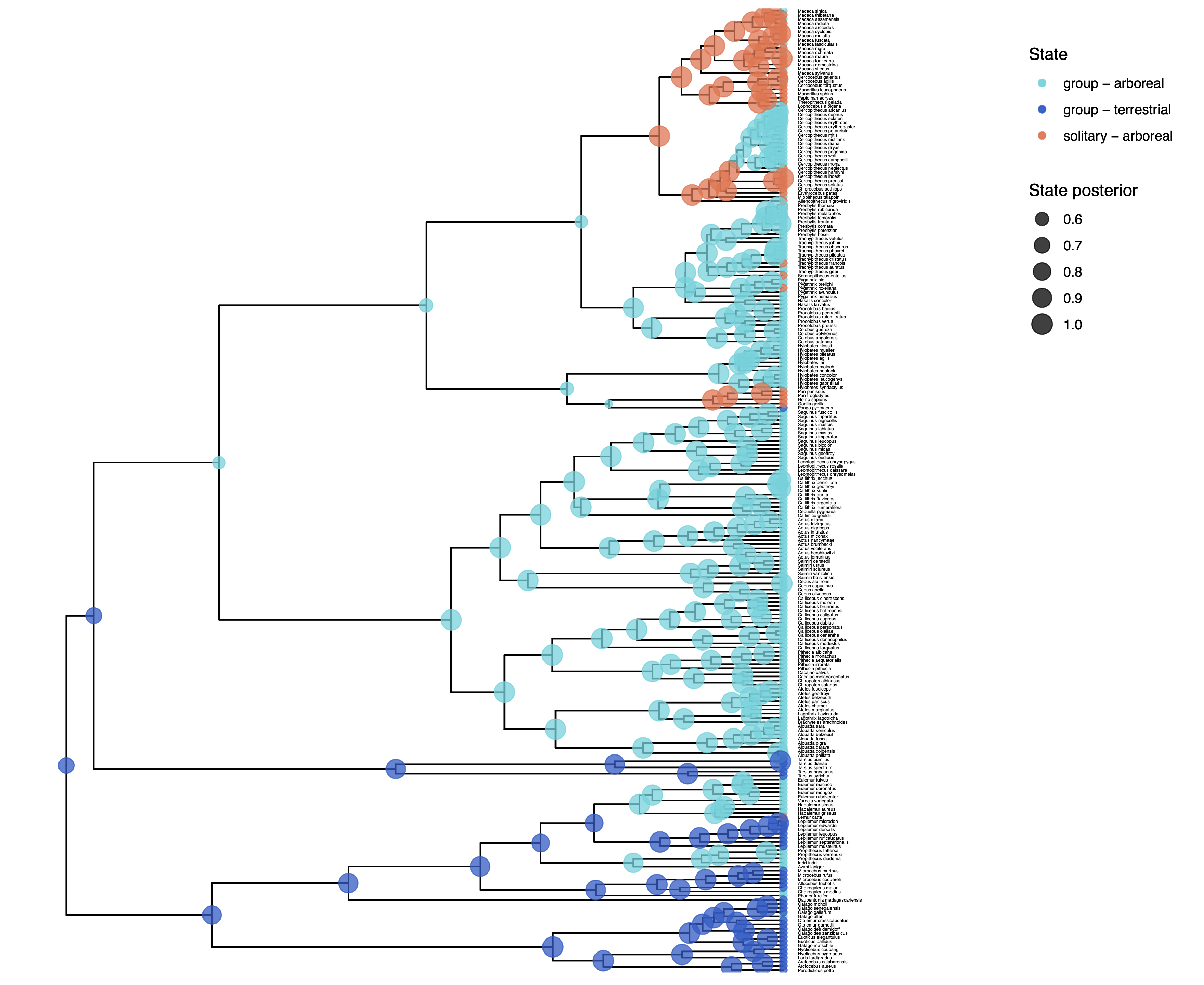
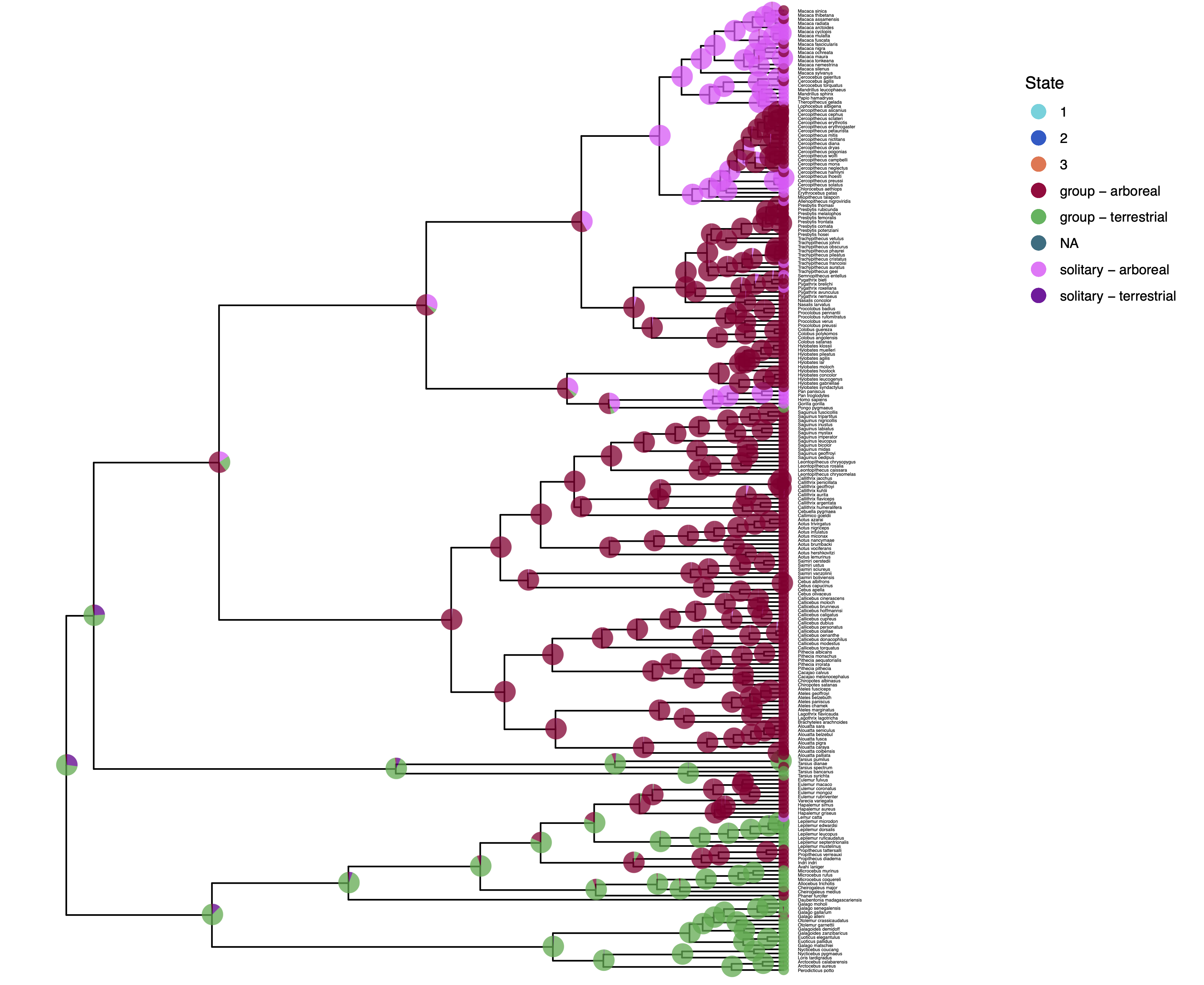
Visualizing Ancestral State Estimates

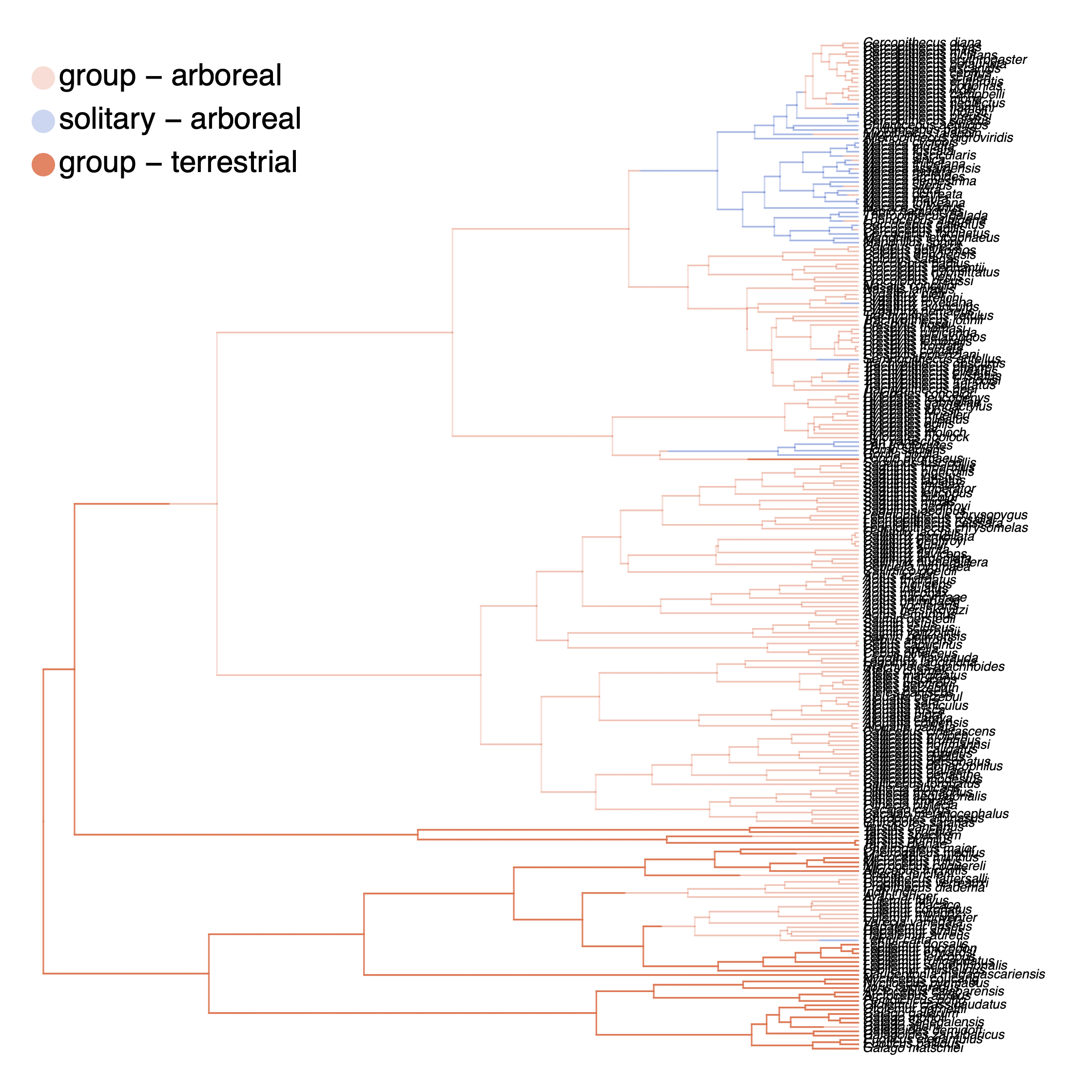
We have previously plotted the ancestral states, both the maximum a posterior (MAP) states as well as the posterior probabilities of all states shown as pie chart Discrete morphology - Ancestral State Estimation. We also showed before how to plot the stochastic character mapping using phytools. My output is shown in .

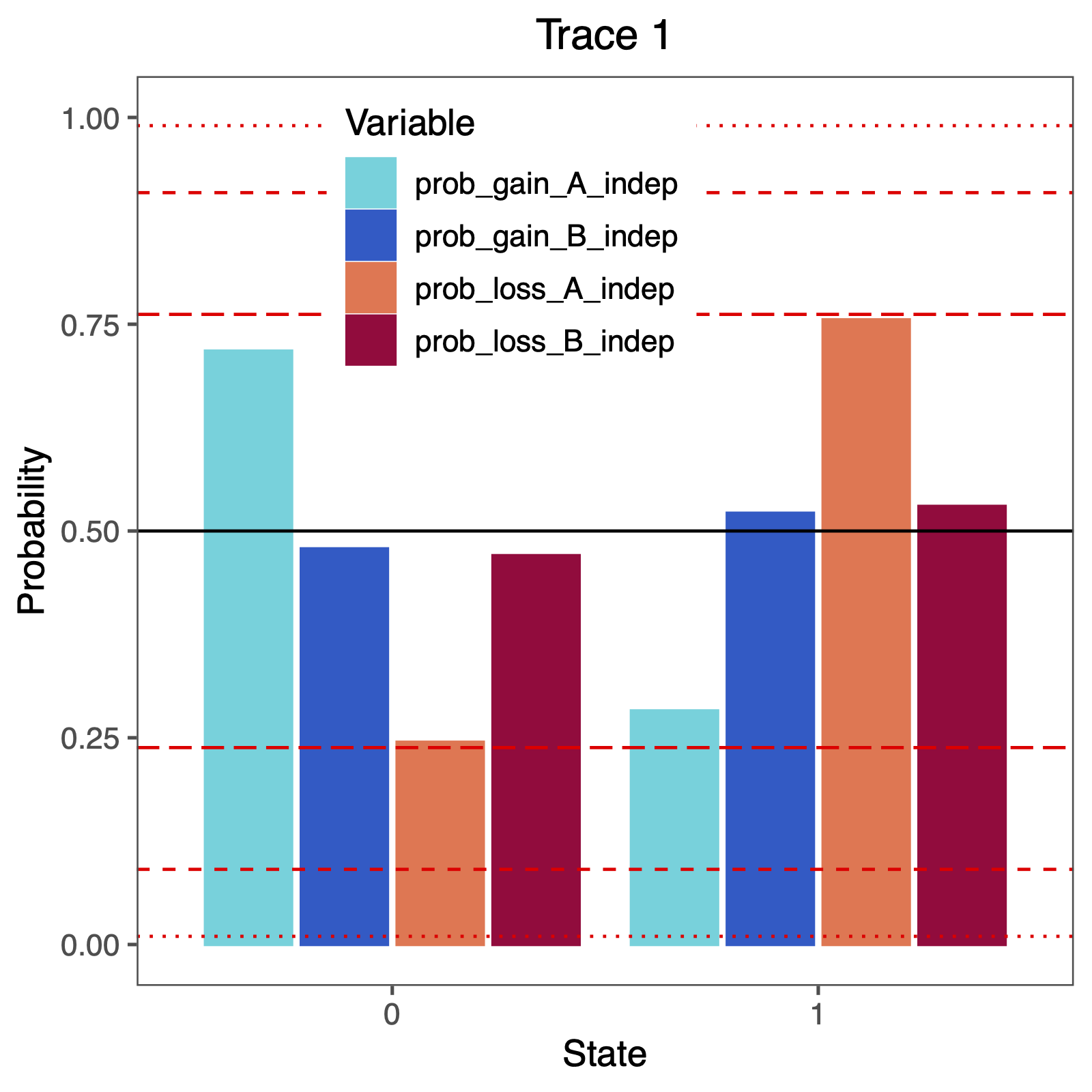
The more important output analysis here is the probability of the rates being dependent or not. Therefore, we will plot the probability that two rates were identical. You can do this nicely in RevGadgets (Tribble et al. 2022)

library(RevGadgets)
library(ggplot2)

CHARACTER_A <- "solitariness"
CHARACTER_B <- "terrestrially"

# specify the input file
file <- paste0("output/",CHARACTER_A,"_",CHARACTER_B,"_corr_RJ.log")

# read the trace and discard burnin
trace_qual <- readTrace(path = file, burnin = 0.25)

BF <- c(3.2, 10, 100)
p = BF/(1+BF)
# produce the plot object, showing the posterior distributions of the rates.
p <- plotTrace(trace = trace_qual,
          vars = c("prob_gain_A_indep", "prob_gain_B_indep", "prob_loss_A_indep", "prob_loss_B_indep"))[[1]] +
          ylim(0,1) +
          geom_hline(yintercept=0.5, linetype="solid", color = "black") +
          geom_hline(yintercept=p, linetype=c("longdash","dashed","dotted"), color = "red") +
          geom_hline(yintercept=1-p, linetype=c("longdash","dashed","dotted"), color = "red") +
     # modify legend location using ggplot2
     theme(legend.position = c(0.40,0.825))

ggsave(paste0("Primates_",CHARACTER_A,"_",CHARACTER_B,"_corr_RJ.pdf"), p, width = 5, height = 5)

How can you explain the observed allocation of clades to the slow and fast rate categories? Do ancestral state estimates match with the stochastic character maps? How certain are we in the ancestral state estimates?

1. Bollback J.P. 2006. SIMMAP: stochastic character mapping of discrete traits on phylogenies. BMC bioinformatics. 7:88.
2. Pagel M., Meade A. 2004. A Phylogenetic Mixture Model for Detecting Pattern-Heterogeneity in Gene Sequence or Character-State Data. Systematic Biology. 53:571–581. 10.1080/10635150490468675
3. Revell L.J. 2012. phytools: an R package for phylogenetic comparative biology (and other things). Methods in Ecology and Evolution.:217–223.
4. Tribble C.M., Freyman W.A., Landis M.J., Lim J.Y., Barido-Sottani J., Kopperud B.T., Höhna S., May M.R. 2022. RevGadgets: An R package for visualizing Bayesian phylogenetic analyses from RevBayes. Methods in Ecology and Evolution. 13:314–323. https://doi.org/10.1111/2041-210X.13750