Polymorphism-aware phylogenetic models

This tutorial comes with a recorded video walkthrough. The video corresponding to each section of the exercise is linked next to the section title. The full playlist is available here:

Polymorphism-aware phylogenetic models

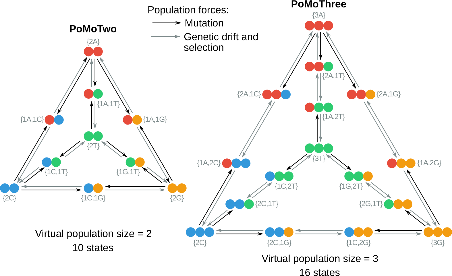
The polymorphism-aware phylogenetic models (PoMos) are alternative approaches to species tree estimation (De Maio et al. 2013) that add a new layer of complexity to the standard substitution models by accounting for population-level forces to describe the process of sequence evolution (De Maio et al. 2015; Schrempf et al. 2016; Borges et al. 2019). PoMos model the evolution of a population of individuals in which changes in allele content (e.g., due to mutations) and frequency (e.g., due to genetic drift or selection) are both possible ().

PoMos stand out from the standard phylogenetic substitution models and other species tree methods because they:

• permit to disentangle the contribution of evolutionary forces to the evolutionary process (e.g., genetic drift, mutational biases, and selection);
• consider polymorphisms, thus permitting inferences with data from multiple individuals and populations;
• naturally account for incomplete lineage sorting (i.e., the persistence of ancestral polymorphisms during speciation events), a known process of phylogenetic discord;
• directly estimate the species tree and is computationally efficient by circumventing the many constraints between the species tree and the genealogical histories.

Overall, PoMos constitute a full-likelihood yet computationally efficient approach to species tree inference. PoMos are designed to cope with recent radiations, including incomplete lineage sorting, and long divergence times.

Polymorphism-aware phylogenetic models: the model

PoMos model the evolution of a population of $N$ individuals and $K$ alleles in which changes in allele content and frequency occur. These are mediated by population forces such as mutation, genetic drift, and selection. The PoMo state-space includes fixed (or boundary) states \(\{Na_i\}\), in which all $N$ individuals have the same allele \(i \in \{0,1,...,K-1\}\), and polymorphic states \(\{na_i,(N-n)a_j\}\), in which two alleles $a_i$ and $a_j$ are present in the population with absolute frequencies $n$ and $N-n$.

• Mutations occur with rate $\mu_{a_ia_j}$. Mutations govern the allele content and only occur in the fixed states: \(q_{\{Na_i\} \rightarrow \{(N-1)a_i,1a_j\}}=\mu_{a_ia_j} \label{equation1}\tag{1}\) Often, a reversible mutational model is considered. In this case, we break the mutations into a base composition $\pi$ and exchangeability parameter $\rho$ (i.e., $\mu_{a_ia_j}=\rho_{a_ia_j}\pi_{a_j}$) just like the GTR. However, in PoMos, these do not represent substitutions but mutations. Such an assumption can still model mutational biases quite well and simplifies obtaining formal quantities with PoMos. Another assumption of PoMos is that mutations can only occur in fixed states. This corresponds to the assumption that mutation rates are low, which is verified for the majority of multicellular eukaryotes.
• Genetic drift is modeled according to the Moran model, in which one individual is chosen to die and one individual is chosen to reproduce at each time step. Selection acts to (dis)favor alleles by differentiated fitnesses: $\phi_{a_i}$. Together, genetic drift and selection govern the allele frequency changes: \(q_{\{na_i,(N-n)a_j\} \rightarrow \{(n+1)a_i,(N-n-1)a_j\}}=\frac{n(N-n)}{N}\phi_{a_i} \label{equation2}\tag{2}\)

Like the standard substitution models, PoMos are continuous-time Markov models and are fully characterized by their rate matrices. The rates in \ref{equation1} and \ref{equation2} define the PoMos rate matrices. RevBayes includes a plethora of PoMo rate matrices that permit modeling population dynamics with any number of alleles, reversible mutations (i.e., $\mu_{a_ia_j}=\rho_{a_ia_j}\pi_{a_j}$) and selection. These are described in .

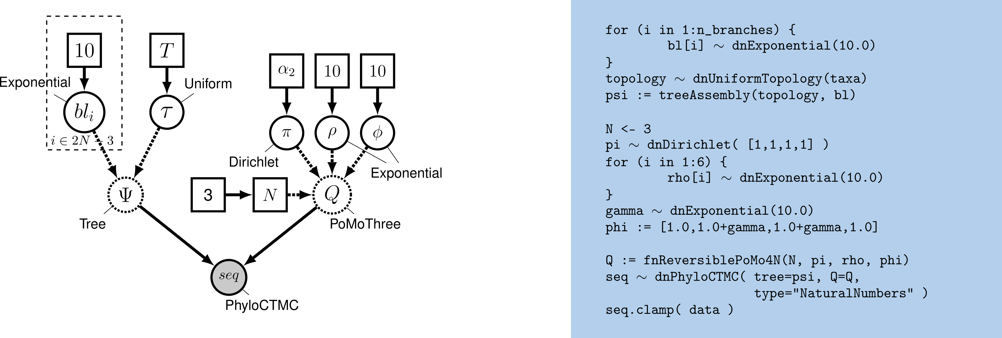
This tutorial demonstrates how to set up and perform analyses using polymorphism-aware phylogenetic models. You will perform phylogeny inference using the virtual PoMos Two and Three. These models allow for very efficient species tree inferences under neutrality (PoMoTwo) and selection (PoMoThree) because they operate on a smaller state space (missing reference). You will perform a Markov chain Monte Carlo (MCMC) analysis to estimate phylogeny and other model parameters. The graphical model representation under PoMoThree is depicted in figure .

Count files

PoMos perform inferences based on allele frequency data. Count files are the files where we store such data. They contain two header lines. The first line indicates the number of taxa and the number of sites (or loci) in the sequence alignment. You might have noticed that NPOP stands for the number of populations, but this is not necessarily the case. PoMos can be employed to infer the evolutionary history of different species or even other systematic units that one might be interested in studying (e.g., subspecies, communities, etc.).

A second line states the genomic position of every locus (chromosome and location) and the taxon names. The first two columns are not used for inference, which means that if you are working with taxa for which such information is not available, you can input these columns with dummy values (e.g., NA or ?). All the other lines in the count file include allelic counts separated by commas. White spaces separate all the elements in the count file. Let us have a look at some lines of the great ape count file we will analyze in this tutorial:

COUNTSFILE NPOP 3 NSITES 5
CHROM POS       Gorilla_beringei_graueri Gorilla_gorilla_dielhi Gorilla_gorilla_gorilla
chr1  41275799  6,0,0,0                  2,0,0,0                54,0,0,0 
chr2  120104878 6,0,0,0                  2,0,0,0                54,0,0,0 
chr11 61364549  0,6,0,0                  0,2,0,0                0,54,0,0 
chr17 44837427  6,0,0,0                  2,0,0,0                54,0,0,0 
chr19 7495905   4,0,2,0                  2,0,0,0                10,0,44,0 

The four allelic counts in this count file represent the allelic counts of the A, C, G, and T, respectively. Thus, we know that the Gorilla_gorilla_gorilla has an AG polymorphism at position 7 495 905 of chromosome 19. The allele order in the allelic counts can be any. However, you have to keep in mind that the vector of mutation rates, exchangeabilities, base frequencies, and fitness coefficients all follow the order of the allele counts in the count file:

• the base frequencies and the fitness vectors are in the same order as in the counts: i.e., \(\{a_0,a_1,...,a_{K-1}\}\);
• the vector mutation rates (this vector is used in the non-reversible models) are \(\{a_0a_1, a_1a_0, a_0a_2, a_2a_0,...\}\);
• the vector of exchangeabilities follows a similar pattern as for the mutation rates, but without the reversed mutation: i.e., \(\{a_0a_1, a_0a_2, ...\}\).

Loading the data

The first step in this tutorial is to convert the allelic counts into PoMo states. Open the terminal and place it in your working directory, let us call it PoMos, but you can use a name of your preference. Inside PoMos create the usual data and output folders. Before starting to actually load the data, run RevBayes by typing ./rb (or ./rb-mpi) in the console. Open the great_apes_pomothree.Rev file using an appropriate text editor so you can follow what each command is doing. Once you know what this .Rev script is doing in detail, you can automatically run it as follows:

./rb great_apes_pomothree.Rev

We mentioned previously that the PoMo state space includes fixed and polymorphic states. However, allele counts are samples of (usually) a few individuals from the population. For example, sampled fixed sites might not necessarily be fixed in the original population. We might just have been unlucky and only sampled individuals with the same allele from a locus that is polymorphic. It is typically the case that real genetic diversity is undersampled in population genetic studies. The fewer the number of sampled individuals or the rarer the alleles in the original population (i.e., singletons or doubletons), the more likely we are to observe fake fixed sites in the sequence alignment. There are methods that help us correct for such bias by attributing to each of the allelic counts an appropriate PoMo state. One such method is the weighted-method (Schrempf et al. 2016), which weights each PoMo state based on binomial sampling. This is automatically done in RevBayes when we use  the function readPoMoCountFile. We just need to define the location of the counts file, the virtual population size, which, as we will be using the virtual PoMo three for inferences, we set to 3, and the data type format, which is PoMo.

N <- 3
data <- readPoMoCountFile(countFile="data/great_apes_1000.cf", virtualPopulationSize=N, format="PoMo")

Information about the alignment can be obtained by typing data. 

>data
   PoMo character matrix with 12 taxa and 1000 characters
   ======================================================
   Origination:                   
   Number of taxa:                12
   Number of included taxa:       12
   Number of characters:          1000
   Number of included characters: 1000
   Datatype:                      PoMo

If, instead of a count file, you have a list of sequences per individual (either in a fasta or nexus file), RevBayes can still convert it to PoMo data format. To do that, you will need to read the sequences, provide a file with the taxon names, and then perform the conversion to the PoMo state space with pomoStateConver. To identify individual sequences as belonging to the same taxon, just use the same name. These are the commands you will need:

data_char = readDiscreteCharacterData("data/individual_sequences.nex")
taxa = readTaxonData("data/taxon_names.txt")
data = pomoStateConvert(aln=data_char, k=4, virtualNe=N, taxa)

Next, we will specify some useful variables. These include the number of taxa, taxa names, and the number of branches. We will need that information for setting up our model in subsequent steps.

n_taxa     <- data.ntaxa()
n_branches <- 2*n_taxa-3
taxa       <- data.taxa()

Additionally, we set up a variable that holds all the moves and monitors them for our analysis. Recall that moves are algorithms used to propose new parameter values during the MCMC simulation. Monitors print the values of model parameters to the screen and/or log files during the MCMC analysis.

moves    = VectorMoves()  
monitors = VectorMonitors()

Setting up the model

Estimating an unrooted tree under the virtual PoMos requires specifying two main components:

• the PoMo model, which in our case is PoMoTwo or PoMoThree;
• the tree topology and branch lengths.

A given PoMo model is defined by its corresponding instantaneous-rate matrix, Q. PoMoTwo and PoMoThree have three free parameters in common: the population size N, the allele frequencies pi, and the exchangeabilities rho. PoMoThree additionally includes the allele fitnesses phi, as it accounts for selection. We will set up the virtual PoMoTwo and Three using the function fnReversiblePoMo4N. You can check the input parameters of any PoMo function by typing its name right after the question mark: ?fnReversiblePoMo4N.

As expected, this function has as input parameters the population size N, base frequencies, exchangeabilities rho and fitnesses phi. We will first set out the PoMoThree, which we can do by setting $N$ to 3. Similarly, if you wanted to set out the neutral PoMo (i.e., PoMoTwo), you could set N to 2 instead. Thus, N is a fixed node, as we had previously defined. 

Since pi, rho, and gamma are stochastic variables, we must specify a move to propose updates to them. A good move on variables drawn from a Dirichlet distribution (i.e., pi) is the mvBetaSimplex. This move randomly takes an element from the allele frequencies vector pi, proposes a new value drawn from a beta distribution, and then rescales all values to sum to 1. The weight option inside the moves specifies how often the move will be applied, either on average per iteration or relative to all other moves.

# allele frequencies
pi_prior <- [1,1,1,1]
pi ~ dnDirichlet(pi_prior)
moves.append( mvBetaSimplex(pi, weight=2) )

The rho and phi parameters must be a positive real number and a natural choice for their prior distributions is the exponential distribution. Again, we need to specify a move for these stochastic variables, and a simple scaling move mvScale typically works. In this tutorial, we want our model to capture the effect of GC-bias gene conversion. For that, we define gamma, which will represent the GC-bias rate. The allele fitnesses phi of G and C will thus be represented by gamma, while those of A and T by 1.0. Note that phi is a deterministic node that depends on the GC-bias rate gamma.

# exchangeabilities
for (i in 1:6){
  rho[i] ~ dnExponential(10.0)
  moves.append(mvScale( rho[i], weight=2 ))
}

# fitness coefficients
gamma ~ dnExponential(1.0)
moves.append(mvScale( gamma, weight=2 ))
phi := [1.0,1.0+gamma,1.0+gamma,1.0]

The function fnReversiblePoMo4N will create an instantaneous-rate matrix.

# rate matrix
Q := fnReversiblePoMo4N(N,pi,rho,phi)

An important note: We could similarly have used the functions fnReversiblePoMoTwo4N and fnReversiblePoMoThree4N, to set the rate matrices. These are particularly useful when one has information about mutation or the GC-bias gene conversion rate (for some model organisms, this information might be available) and wants to include it via informative priors. In such a case, the population size is not a fixed node, and it can be jointly estimated. In this tutorial, we are assuming that no prior information is available for the mutation or GC-bias rates. Note that selection is not identifiable with two virtual individuals, so the vector of fitness coefficients cannot be inputted for the fnReversiblePoMoTwo4N: it is by default equal to the unitary vector (i.e., the neutral scenario). To check the input parameters of PoMoTwo, you can type ?fnReversiblePoMoTwo4N ; you will see that the fitness coefficient phi is missing. As a consequence, if we want to employ the PoMoTwo model with the general fnReversiblePoMoTwo4N, we have to set the fitness coefficients to 1.0.

The tree topology and branch lengths are stochastic nodes in our phylogenetic model. We will assume that all possible labeled, unrooted tree topologies have equal probability. In the case of an unrooted tree topology, we use the nearest-neighbor interchange move mvNNI (a subtree-prune and regrafting move mvSPR could also be used).

# topology
topology ~ dnUniformTopology(taxa)
moves.append( mvNNI(topology, weight=2*n_taxa) )

Next, we have to create a stochastic node representing the length of each of the 2*n_taxa−3 branches in our tree. We can do this using a for loop. In this loop, we can create each of the branch-length nodes and assign each move.

# branch lengths
for (i in 1:n_branches) {
   branch_lengths[i] ~ dnExponential(10.0)
   moves.append( mvScale(branch_lengths[i]) )
}

Finally, we combine the tree topology and branch lengths. We do this using the treeAssembly function, which applies the value of the ith member of the branch_lengths vector to the branch leading to the ith node in the topology. Thus, the psi variable is a deterministic node:

psi := treeAssembly(topology, branch_lengths)

We have fully specified all of the parameters of our phylogenetic model:

• the tree with branch lengths of psi;
• the PoMo instantaneous-rate matrix Q;
• the type of character data: i.e., PoMo.

Collectively, these parameters comprise a distribution called the phylogenetic continuous-time Markov chain, and we use the dnPhyloCTMC function to create this node. This distribution requires several input arguments:

sequences ~ dnPhyloCTMC(psi,Q=Q,type="PoMo")

Once the PhyloCTMC model has been created, we can attach our sequence data to the tip nodes in the tree. Although we assume that our sequence data are random variables, they are realizations of our phylogenetic model. For inference purposes, we assume that the sequence data are clamped to their observed values.

sequences.clamp(data)

When this function is called, RevBayes sets each of the stochastic nodes representing the tree’s tips to the corresponding nucleotide sequence in the alignment. This essentially tells the program that we have observed sequence data at the tree tips.

Finally, we wrap the entire model in a single object. To do this, we only need to give the model function a single node.

pomo_model = model(pi)

Setting, running, and summarizing the MCMC simulation

For our MCMC analysis, we need to set up a vector of monitors to record the states of our Markov chain. First, we will initialize the model monitor using the mnModel function. This creates a new monitor variable that will output the states for all model parameters when passed into an MCMC function. We will sample every 10th generation, and the resulting file can be found in the output folder.

monitors.append( mnModel(filename="output/great_apes_pomothree.log", printgen=10) )

The mnFile monitor will record the states for only the parameters passed in as arguments. We use this monitor to specify the output for our sampled trees and branch lengths. Again, we sample every 10th generation.

monitors.append( mnFile(filename="output/great_apes_pomothree.trees", printgen=10, psi) )

Finally, create a screen monitor that will report the states of specified variables to the screen with mnScreen. This monitor mostly helps us follow the progress of the MCMC run.

monitors.append( mnScreen(printgen=10) )

With a fully specified model, a set of monitors, and a set of moves, we can now set up the MCMC algorithm that will sample parameter values in proportion to their posterior probability. The mcmc function will create our MCMC object. Furthermore, we will perform two independent MCMC runs to ensure proper convergence and mixing.

pomo_mcmc = mcmc(pomo_model, monitors, moves, nruns=2, combine="mixed")

Now, we can start the MCMC.

pomo_mcmc.run( generations=10000 )

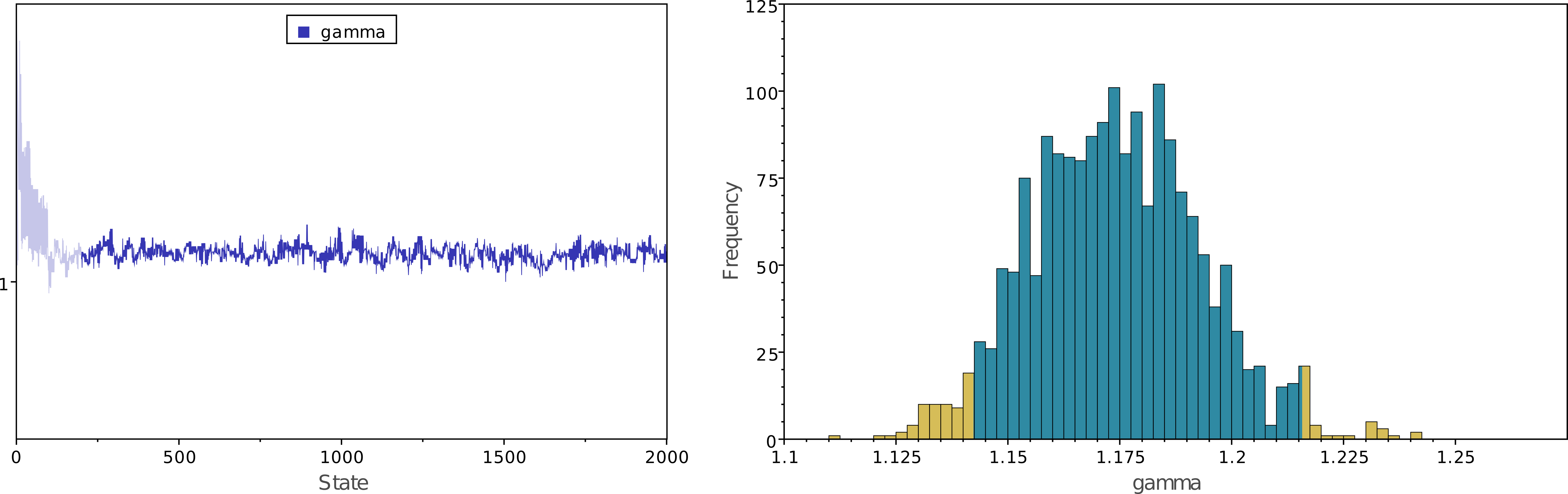
When the analysis is complete, you will have the monitored files in your output directory. Software like Tracer or the R package Convenient allow evaluating convergence and mixing. Look at the file called output/great_apes_pomothree.log in Tracer. There you see the posterior distribution of the continuous parameters. Let us look at the posterior distribution of the GC-bias rate $\gamma$. Is there any evidence of GC-bias in these great apes sequences?

Apart from the continuous parameters, we need to summarize the trees sampled from the posterior distribution. RevBayes can summarize the sampled trees by reading in the tree trace file:

trace = readTreeTrace("output/great_apes_pomothree.trees", treetype="non-clock", burnin= 0.2)

The mapTree function will summarize the tree samples and write the maximum a posteriori (MAP) tree to the specified file. The MAP tree can be found in the output folder.

mapTree(trace, file="output/great_apes_pomothree_MAP.tree" )

Look at the file called output/great_apes_pomothree_MAP.tree and open it in FigTree. The maximum a posteriori estimate of the great ape phylogeny under the PoMoThree model should look like that of .

Some questions

1. What is the GC-bias rate (this is the selection coefficient) for the great ape populations? Rescale to its real value by assuming that the great apes have an effective population size of about 10 000 individuals. You should use the relation $(1+\gamma’)^{M-1}=(1+\gamma)^{N-1}$ to rescale $\gamma$.  $M$ and $N$ are the virtual and effective population sizes, and $\gamma’$ and $\gamma$ are the GC-bias rates on the virtual and effective populations.

2. With as your guide, draw the probabilistic graphical model of the PoMoTwo model.

3. What changes have to be made to the great_apes_pomothree.Rev to make inferences under the PoMoTwo model?

4. Run an MCMC analysis to estimate the posterior distribution under the PoMoTwo model. Are the resulting estimates of the mutation rates (base frequencies and exchangeabilities) equal? If not, how much do they differ?

5. Compare the MAP trees estimated under PoMoTwo and PoMoThree. Are they equal, and if not, how much do they differ?

1. Borges R., Boussau B., Höhna S., Pereira R.J., Kosiol C. 2022. Polymorphism‐aware estimation of species trees and evolutionary forces from genomic sequences with RevBayes. Methods in Ecology and Evolution. 10.1111/2041-210X.13980
2. Borges R., Szöllősi G.J., Kosiol C. 2019. Quantifying GC-Biased Gene Conversion in Great Ape Genomes Using Polymorphism-Aware Models. Genetics. 212:1321–1336. 10.1534/genetics.119.302074
3. Höhna S., Heath T.A., Boussau B., Landis M.J., Ronquist F., Huelsenbeck J.P. 2014. Probabilistic Graphical Model Representation in Phylogenetics. Systematic Biology. 63:753–771. 10.1093/sysbio/syu039
4. Schrempf D., Minh B.Q., De Maio N., Haeseler A. von, Kosiol C. 2016. Reversible polymorphism-aware phylogenetic models and their application to tree inference. Journal of Theoretical Biology. 407:362–370. 10.1016/j.jtbi.2016.07.042
5. De Maio N., Schlötterer C., Kosiol C. 2013. Linking great apes genome evolution across time scales using polymorphism-aware phylogenetic models. 30:2249–2262. 10.1093/molbev/mst131
6. De Maio N., Schrempf D., Kosiol C. 2015. PoMo: An Allele Frequency-Based Approach for Species Tree Estimation. Systematic Biology. 64:1018–1031. 10.1093/sysbio/syv048