Overview
This tutorial describes how to specify an episodic birth-death model in RevBayes (Höhna et al. 2016).
The episodic birth-death model is a process where diversification rates vary episodically through time
and are modeled as piecewise-constant rates (Stadler 2011; Höhna 2015).
The probabilistic graphical model is given once at the beginning of this tutorial.
Your goal is to estimate speciation and extinction rates through-time using
Markov chain Monte Carlo (MCMC).
You should read first the Introduction to Diversification Rate Estimation which explains the theory and gives some general overview of diversification rate estimation and Simple Diversification Rate Estimation which goes through a very simple pure birth and birth-death model for estimating diversification rates.
Episodic Diversification Rate Models
The basic idea behind the model is that speciation and extinction rates are constant within time intervals but can be different between time intervals. Thus, we will divide time into equally sized intervals. An overview of the underlying theory of the specific model and implementation is given in Höhna (2015), Magee and Höhna (2021).
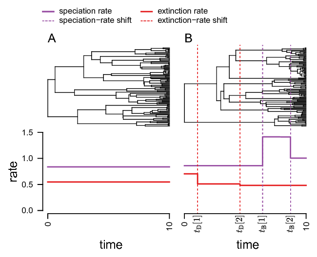
shows an example of a constant rate birth-death process and an episodic birth-death process.
We assume that the log-transformed rates follow a Horseshoe Markov random field (HSMRF) prior distribution Magee et al. (2020). This prior assumes that rates are autocorrelated, that is, rates in the current time interval will be centered around the rates in the previous time interval. The assumption of autocorrelated rates does not only makes sense biologically but also improves our ability to estimate parameters. The HSMRF allows for periods of relatively constant rates interspersed with large jumps, and can be used with large numbers of intervals (hundreds) to provide fine-scale detail in estimated rates.
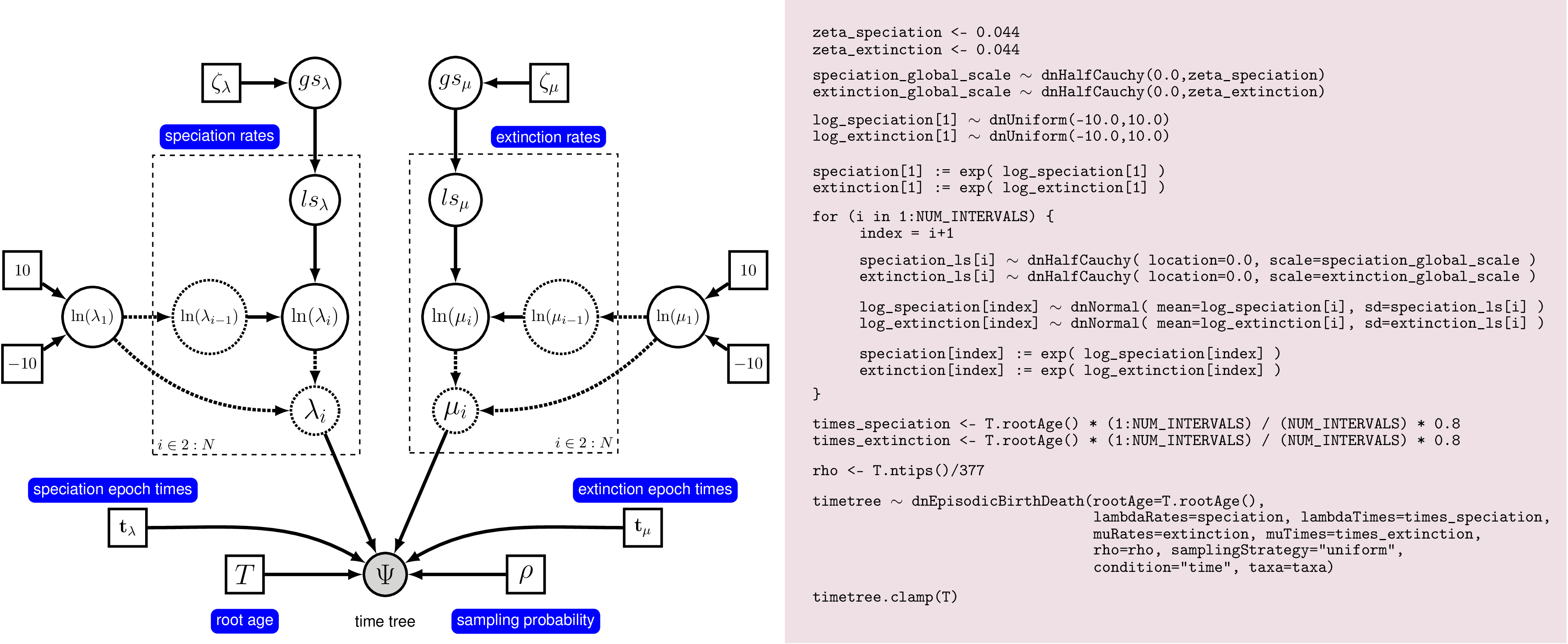
Rev code. On the left we see a
graphical model describing the HSMRF model for rate-variation through time.
On the right we show the corresponding Rev commands to instantiate this model.
This figure gives a complete overview of the model that we use here in this analysis.
There are many ways to represent the HSMRF model, this one is easy to read, but
more computationally burdensome than the version we will use in practice.We show an idealized graphical model of the episodic birth-death process with autocorrelated rates in . This graphical model shows you which variables are included in the model, and the dependency between the variables. Thus, it makes the structure and assumption of the model clear and visible instead of a black-box (Höhna et al. 2014). For example, you see how the speciation and extinction rates in each time interval depend on the rates of the previous interval, and that we use a hyperprior for the standard deviation of rates between time intervals. Note that the actual set up of the plates in Rev code will appear to differ from what is shown here. This is because there are many ways to represent the HSMRF model, and with some small re-parameterization and a function to replace the plate(s), we can make it run much more efficiently and easily in MCMC.
Estimating Episodic Diversification Rates
Read the tree
Begin by reading in the “observed” tree.
T <- readTrees("data/primates_tree.nex")[1]
From this tree, we get some helpful variables, such as the taxon information which we need to instantiate the birth-death process.
taxa <- T.taxa()
Additionally, we initialize a variable for our vector of moves and monitors.
moves    = VectorMoves()
monitors = VectorMonitors()
Finally, we create a helper variable that specifies the number of intervals.
NUM_INTERVALS = 10
NUM_BREAKS := NUM_INTERVALS - 1
Using this variable we can easily change our script to break-up time into many (e.g., NUM_INTERVALS = 100).
Specifying the model
Priors on amount of rate variation
We start by specifying prior distributions on the rates.
The overall model is a HSMRF birth-death model.
In this model, the changes in log-scale rates between intervals follow a Horseshoe distribution (Carvalho et al. 2010), which allows for large jumps in rate while assuming most changes are very small.
We need a parameter to control the overall variability from present to past in the diversification rates, the global scale parameter.
We must also set the global scale hyperprior, which acts with the global scale parameter to set the prior on rate variability.
In this example, we use 10 speciation and extinction rate intervals, but the HSMRF enables us to use much larger numbers.
The global scale hyperprior should be set based on how many intervals are used, in the case of 100 intervals, use 0.0021.
RevGadgets provides the function setMRFGlobalScaleHyperpriorNShifts() to compute this parameter for other numbers of intervals.
speciation_global_scale_hyperprior <- 0.044
extinction_global_scale_hyperprior <- 0.044

speciation_global_scale ~ dnHalfCauchy(0,1)
extinction_global_scale ~ dnHalfCauchy(0,1)
Specifying episodic rates
As we mentioned before, we will apply HSMRF distributions as prior for the log-transformed speciation and extinction rates. We begin with the rates at the present which is our initial rate parameter. The rates at the present will be specified slightly differently because they are not correlated to any previous rates. This is because we are actually modeling rate-changes backwards in time and there is no previous rate for the rate at the present. Modeling rates backwards in time makes it easier for us if we had some prior information about some event affected diversification sometime before the present, e.g., 25 million years ago.
We use a uniform distribution between -10 and 10 because of our lack of prior knowledge on the diversification rate. This actually means that we allow speciation and extinction rates between $e^{-10}$ and $e^{10}$, so we should clearly cover the true values. (Note that for diversification rate estimates, $e^{-10}$ is virtually 0 since the rate is so slow).
log_speciation_at_present ~ dnUniform(-10.0,10.0)
log_speciation_at_present.setValue(0.0)
log_extinction_at_present ~ dnUniform(-10.0,10.0)
log_extinction_at_present.setValue(-1.0)
We apply efficient sliding moves to each parameter.
moves.append( mvScaleBactrian(log_speciation_at_present,weight=5))
moves.append( mvScaleBactrian(log_extinction_at_present,weight=5))
To make MCMC possible for the HSMRF model, we use what is called a non-centered parameterization.
This means that first we specify the log-scale changes in rate between intervals, and later we assemble these into the vector of rates, by adding them together and then exponentiating.
The HSMRF also requires a vector of local scale parameters.
These give the HSMRF a property called local adaptivity, which allow it to have rapidly varying rates in some intervals and nearly constant rates in others.
This can be done efficiently using a for-loop.
for (i in 1:NUM_BREAKS) {
  sigma_speciation[i] ~ dnHalfCauchy(0,1)
  sigma_extinction[i] ~ dnHalfCauchy(0,1)

  # Make sure values initialize to something reasonable
  sigma_speciation[i].setValue(runif(1,0.005,0.1)[1])
  sigma_extinction[i].setValue(runif(1,0.005,0.1)[1])

  # non-centralized parameterization of horseshoe
  delta_log_speciation[i] ~ dnNormal( mean=0, sd=sigma_speciation[i]*speciation_global_scale*speciation_global_scale_hyperprior )
  delta_log_extinction[i] ~ dnNormal( mean=0, sd=sigma_extinction[i]*extinction_global_scale*extinction_global_scale_hyperprior )
}
Now, we take the pieces we have for the rates (the global and local scales, the rate at the present, and the log-changes) and we assemble the overall rates.
The delta parameters are differences in log-scale rates, and so we need to sum them then exponentiate.
For example, speciation[2] := exp(log_speciation_at_present + delta_log_speciation[1]).
Because the sd values for any of the log-scale differences is equivalent to what we wrote in the DAG above (simply written in expanded form), the model here is equivalent to the one in the DAG.
The function fnassembleContinuousMRF() does all the summation and exponentiation efficiently for all speciation and extinction rates in all intervals and avoids making the DAG too big.
speciation := fnassembleContinuousMRF(log_speciation_at_present,delta_log_speciation,initialValueIsLogScale=TRUE,order=1)
extinction := fnassembleContinuousMRF(log_extinction_at_present,delta_log_extinction,initialValueIsLogScale=TRUE,order=1)
The HSMRF requires a unique set of MCMC samplers to work. While you can place individual moves on the local and global scales and the log-changes, adequate MCMC sampling requires moves that exploit the structure of the model. These moves are the elliptical slice sampler that works on the log-changes, a Gibbs sampler for the global and local scales, and a recommended swap move (that works on both). But these moves require us to have the HSMRF model written out this way, and not the version we showed in the DAG.
# Move all field parameters in one go
moves.append( mvEllipticalSliceSamplingSimple(delta_log_speciation,weight=5,tune=FALSE) )
moves.append( mvEllipticalSliceSamplingSimple(delta_log_extinction,weight=5,tune=FALSE) )

# Move all field hyperparameters in one go
moves.append( mvHSRFHyperpriorsGibbs(speciation_global_scale, sigma_speciation , delta_log_speciation , speciation_global_scale_hyperprior, propGlobalOnly=0.75, weight=10) )
moves.append( mvHSRFHyperpriorsGibbs(extinction_global_scale, sigma_extinction , delta_log_extinction , extinction_global_scale_hyperprior, propGlobalOnly=0.75, weight=10) )

# Swap moves to exchange adjacent delta,sigma pairs
moves.append( mvHSRFIntervalSwap(delta_log_speciation ,sigma_speciation ,weight=5) )
moves.append( mvHSRFIntervalSwap(delta_log_extinction ,sigma_extinction ,weight=5) )
Setting up the time intervals
The model formulation we are using assumes that time points are evenly spaced. We must now create this vector of times to give to the birth death model.
interval_times <- abs(T.rootAge() * seq(1, NUM_BREAKS, 1)/NUM_INTERVALS)
This vector of times will be used for both the speciation and extinction rates. Also, remember that the times of the intervals represent ages going backwards in time.
Incomplete Taxon Sampling
We know that we have sampled 233 out of 367 living primate species. To account for this we can set the sampling parameter as a constant node with a value of 233/367. For simplicity, and since almost all species have been sampled, we assume uniform taxon sampling (Höhna et al. 2011; Höhna 2014),
rho <- T.ntips()/367
Root age
The birth-death process requires a parameter for the root age. In this exercise we use a fixed tree and thus we know the age of the tree. Hence, we can get the value for the root from the Magnuson-Ford and Otto (2012) tree.
root_time <- T.rootAge()
The time tree
Now we have all of the parameters we need to specify the full episodic birth-death model. We initialize the stochastic node representing the time tree.
timetree ~ dnEpisodicBirthDeath(rootAge=T.rootAge(), lambdaRates=speciation, lambdaTimes=interval_times, muRates=extinction, muTimes=interval_times, rho=rho, samplingStrategy="uniform", condition="survival", taxa=taxa)
You may notice that we explicitly specify that we want to condition on survival. It is possible to change this condition to the time of the process or the number of sampled taxa too.
Then we attach data to the timetree variable.
timetree.clamp(T)
Finally, we create a workspace object of our whole model using the model() function.
mymodel = model(speciation)
The model() function traversed all of the connections and found all of the nodes we specified.
Running an MCMC analysis
Specifying Monitors
For our MCMC analysis, we need to set up a vector of monitors to record the states of our Markov chain.
First, we will initialize the model monitor using the mnModel function.
This creates a new monitor variable that will output the states for all model parameters
when passed into a MCMC function.
monitors.append( mnModel(filename="output/primates_EBD.log",printgen=10, separator = TAB) )
Additionally, we create four separate file monitors, one for each vector of speciation and extinction rates and for each speciation and extinction rate epoch (\IE the times when the interval ends). We want to have the speciation and extinction rates stored separately so that we can plot them nicely afterwards.
monitors.append( mnFile(filename="output/primates_EBD_speciation_rates.log",printgen=10, separator = TAB, speciation) )
monitors.append( mnFile(filename="output/primates_EBD_speciation_times.log",printgen=10, separator = TAB, interval_times) )
monitors.append( mnFile(filename="output/primates_EBD_extinction_rates.log",printgen=10, separator = TAB, extinction) )
monitors.append( mnFile(filename="output/primates_EBD_extinction_times.log",printgen=10, separator = TAB, interval_times) )
Finally, we create a screen monitor that will report the states of specified variables
to the screen with mnScreen:
monitors.append( mnScreen(printgen=1000, extinction_global_scale, speciation_global_scale) )
Initializing and Running the MCMC Simulation
With a fully specified model, a set of monitors, and a set of moves,
we can now set up the MCMC algorithm that will sample parameter values in proportion
to their posterior probability.
The mcmc() function will create our MCMC object:
mymcmc = mcmc(mymodel, monitors, moves, nruns=2, combine="mixed")
Now, run the MCMC:
mymcmc.run(generations=50000, tuningInterval=200)
When the analysis is complete, you will have the monitored files in your output directory.
You can then visualize the rates through time using R using our package RevGadgets (Tribble et al. 2022).
If you don’t have the R-package RevGadgets installed, or if you have trouble with the package, then please read the separate tutorial about the package (Introduction to RevGadgets).
Just start R in the main directory for this analysis and then type the following commands:
library(RevGadgets)
# specify the output files
speciation_time_file <- "output/primates_EBD_speciation_times.log"
speciation_rate_file <- "output/primates_EBD_speciation_rates.log"
extinction_time_file <- "output/primates_EBD_extinction_times.log"
extinction_rate_file <- "output/primates_EBD_extinction_rates.log"
# read in and process rates
rates <- processDivRates(speciation_time_log = speciation_time_file,
speciation_rate_log = speciation_rate_file,
extinction_time_log = extinction_time_file,
extinction_rate_log = extinction_rate_file,
burnin = 0.25,
summary = "median")
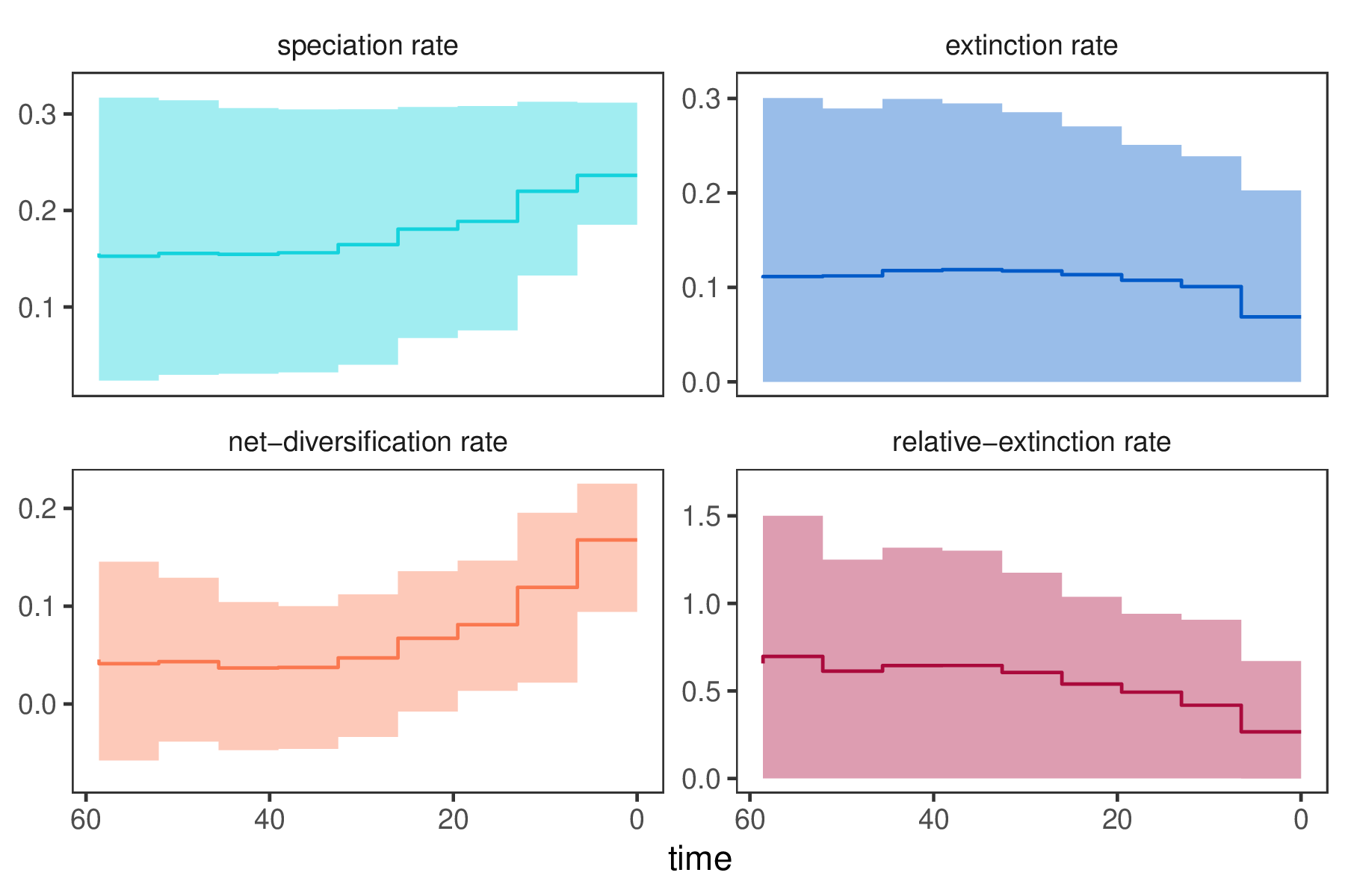
# plot rates through time
p <- plotDivRates(rates = rates) +
xlab("Millions of years ago") +
ylab("Rate per million years")
ggsave("EBD.png", p)
(Note, you may want to add a nice geological timescale to the plot by setting use.geoscale=TRUE but then you can only plot one figure per page.)
⇨ The Rev file for performing this analysis: mcmc_EBD.Rev
Exercise 1
- Run an MCMC simulation to estimate the posterior distribution of the speciation rate and extinction rate.
- Visualize the rate through time using
R. - Do you see evidence for rate decreases or increases? What is the general trend?
- How much faster is the
net-diversificationrate at the present compared to the most ancient time interval? - Is there evidence for rate variation? Look at the estimates of
speciation_global_scaleandextinction_global_scaleinTracer: Is there information in the data to change the estimates from the prior? - Run the analysis using a different number of intervals, e.g., 100 or 200. How do the rates change?
Exercise 2
- In our results we see that the extinction rate is fairly constant. Modify the model by using a constant-rate for the extinction rate parameter but still let the speciation rate vary through time.
- Remove all previous occurrences of the extinction rates (i.e., priors, parameters and moves).
- Specify a lognormal prior distribution on the constant extinction rate (
extinction ~ dnLognormal(-5,sd=2*0.587405)) - Add a move for the new extinction rate parameter
moves.append( mvScaleBactrian(extinction,weight=5.0) ). - Remove the argument
muTimes=interval_timesfrom the birth-death process.
- How does this influence your estimated rates?
Click below to begin the next exercise!
- Carvalho C.M., Polson N.G., Scott J.G. 2010. The horseshoe estimator for sparse signals. Biometrika. 97:465–480.
- Höhna S., Landis M.J., Heath T.A., Boussau B., Lartillot N., Moore B.R., Huelsenbeck J.P., Ronquist F. 2016. RevBayes: Bayesian Phylogenetic Inference Using Graphical Models and an Interactive Model-Specification Language. Systematic Biology. 65:726–736. 10.1093/sysbio/syw021
- Höhna S. 2014. Likelihood Inference of Non-Constant Diversification Rates with Incomplete Taxon Sampling. PLoS One. 9:e84184. 10.1371/journal.pone.0084184
- Höhna S. 2015. The time-dependent reconstructed evolutionary process with a key-role for mass-extinction events. Journal of Theoretical Biology. 380:321–331. http://dx.doi.org/10.1016/j.jtbi.2015.06.005
- Höhna S., Heath T.A., Boussau B., Landis M.J., Ronquist F., Huelsenbeck J.P. 2014. Probabilistic Graphical Model Representation in Phylogenetics. Systematic Biology. 63:753–771. 10.1093/sysbio/syu039
- Höhna S., Stadler T., Ronquist F., Britton T. 2011. Inferring speciation and extinction rates under different species sampling schemes. Molecular Biology and Evolution. 28:2577–2589.
- Magee A.F., Höhna S. 2021. Impact of K-Pg Mass Extinction Event on Crocodylomorpha Inferred from Phylogeny of Extinct and Extant Taxa. bioRxiv.:426715. 10.1101/426715
- Magee A.F., Höhna S., Vasylyeva T.I., Leaché A.D., Minin V.N. 2020. Locally adaptive Bayesian birth-death model successfully detects slow and rapid rate shifts. PLoS Computational Biology. 16:e1007999.
- Magnuson-Ford K., Otto S.P. 2012. Linking the Investigations of Character Evolution and Species Diversification. The American Naturalist. 180:225–245. 10.1086/666649
- Stadler T. 2011. Mammalian phylogeny reveals recent diversification rate shifts. Proceedings of the National Academy of Sciences. 108:6187–6192. 10.1073/pnas.1016876108
- Tribble C.M., Freyman W.A., Landis M.J., Lim J.Y., Barido-Sottani J., Kopperud B.T., Höhna S., May M.R. 2022. RevGadgets: An R package for visualizing Bayesian phylogenetic analyses from RevBayes. Methods in Ecology and Evolution. 13:314–323. https://doi.org/10.1111/2041-210X.13750