Estimating Constant Speciation & Extinction Rates
This tutorial describes how to specify basic birth-death models in RevBayes. Specifically, we will use the pure-birth (Yule; Yule (1925)) process and the constant-rate birth-death process (Kendall 1948; Thompson 1975; Nee et al. 1994). The probabilistic graphical model is given for each component of this tutorial. After each model is specified, you will estimate speciation and extinction rates using Markov chain Monte Carlo (MCMC). Finally, you will estimate the marginal likelihood of the model and evaluate the relative support using Bayes factors.
You should read first the Introduction to Diversification Rate Estimation tutorial, which explains the theory and gives some general overview of diversification rate estimation.
Pure-Birth (Yule) Model
In this section, we will walk through specifying a pure-birth process model and estimating the speciation rate. Then, we will continue by estimating the marginal likelihood of the model so that we can perform model comparison. The section about the birth-death process will be less detailed because it will build up on this section.
The simplest branching model is the pure-birth process described by Yule (1925). Under this model, we assume at any instant in time, every lineage has the same speciation rate, $\lambda$. In its simplest form, the speciation rate remains constant over time. As a result, the waiting time between speciation events is exponential, where the rate of the exponential distribution is the product of the number of extant lineages ($n$) at that time and the speciation rate: $n\lambda$ (Yule 1925; Aldous 2001; Höhna 2015). The pure-birth branching model does not allow for lineage extinction (i.e., the extinction rate $\mu=0$). However, the model depends on a second parameter, $\rho$, which is the probability of sampling a species in the present time. It also depends on the time of the start of the process, whether that is the origin time or root age. Therefore, the probabilistic graphical model of the pure-birth process is quite simple, where the observed time tree topology and node ages are conditional on the speciation rate, sampling probability, and root age ().
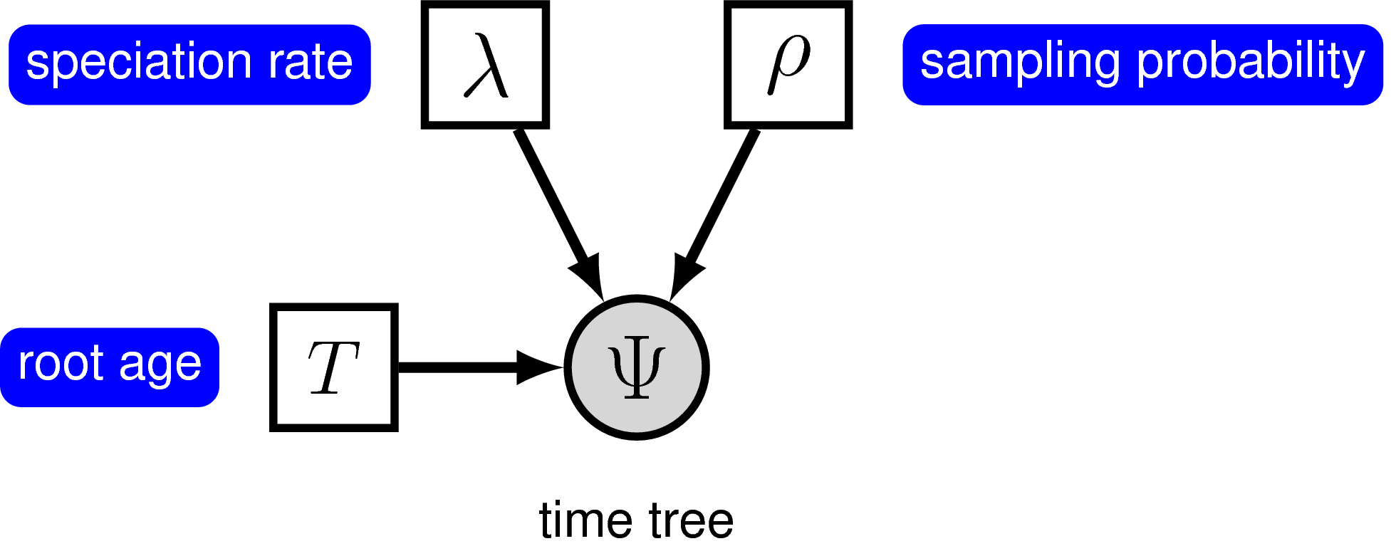
We can add hierarchical structure to this model and account for uncertainty in the value of the speciation rate by placing a prior distribution on $\lambda$ (). The graphical models in and demonstrate the simplicity of the Yule model. Ultimately, the pure birth model is just a special case of the birth-death process, where the extinction rate (typically denoted $\mu$) is a constant node with the value 0.
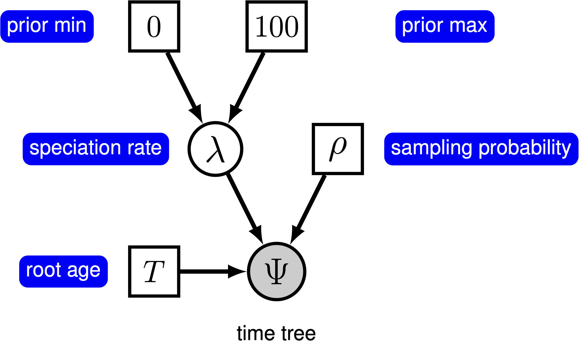
For this exercise, we will specify a Yule model, such that the speciation rate is a stochastic node, drawn from a uniform distribution as in . In a Bayesian framework, we are interested in estimating the posterior probability of $\lambda$ given that we observe a time tree.
\[\begin{equation} \mathbb{P}(\lambda \mid \Psi) = \frac{\mathbb{P}(\Psi \mid \lambda)\mathbb{P}(\lambda \mid \nu)}{\mathbb{P}(\Psi)} \tag{Bayes Theorem}\label{eq:bayes_thereom} \end{equation}\]In this example, we have a phylogeny of 233 primates. We are treating the time tree $\Psi$ as an observation, thus clamping the model with an observed value. The time tree we are conditioning the process on is taken from the analysis by Magnuson-Ford and Otto (2012). Furthermore, there are approximately 367 described primates species, so we will fix the parameter $\rho$ to $233/367$.
⇨ The full Yule-model specification is in the file called mcmc_Yule.Rev.
Read the tree
Begin by reading in the observed tree and get some useful variables. We will need these later on.
T <- readTrees("data/primates_tree.nex")[1]

# Get some useful variables from the data. We need these later on.
taxa <- T.taxa()
Additionally, we can initialize a variable for our vector of moves and monitors:
moves    = VectorMoves()
monitors = VectorMonitors()
Specifying the model
Birth rate
The model we are specifying only has three nodes ().
We can specify the birth rate $\lambda$, the minimum and maximum of the uniform hyperprior on $\lambda$, and the conditional dependency of the two parameters all in one line of Rev code.
birth_rate ~ dnUniform(0,100.0)
Here, the stochastic node called birth_rate represents the speciation rate $\lambda$.
To estimate the value of $\lambda$, we assign a proposal mechanism to operate on this node.
In RevBayes these MCMC sampling algorithms are called moves.
We will use a scaling move on $\lambda$ called mvScale.
moves.append( mvScale(birth_rate,lambda=1.0,tune=true,weight=3.0) )
Sampling probability
Our prior belief is that we have sampled 233 out of 367 living primate species. To account for this we can set the sampling parameter as a constant node with a value of 233/367
rho <- T.ntips()/367
Note that we will assume “uniform” taxon sampling (Höhna et al. 2011; Höhna 2014), which we will specify below. If we want to learn more about different taxon sampling options, then look at Diversification Rate Estimation with Missing Taxa tutorial.
Root age
Any stochastic branching process must be conditioned on a time that represents the start of the process. Typically, this parameter is the origin time and it is assumed that the process started with one lineage. Thus, the origin of a birth-death process is the node that is ancestral to the root node of the tree. For macroevolutionary data, particularly without any sampled fossils, it is difficult to use the origin time. To accommodate this, we can condition on the age of the root by assuming the process started with two lineages that both originate at the time of the root.
We can get the value for the root from the Magnuson-Ford and Otto (2012) tree.
root_time <- T.rootAge()
The time tree
Now we have all of the parameters we need to specify the full pure-birth
model. We can initialize the stochastic node representing the time tree.
Note that we set the mu parameter to the constant value 0.0.
timetree ~ dnBDP(lambda=birth_rate, mu=0.0, rho=rho, rootAge=root_time, samplingStrategy="uniform", condition="survival", taxa=taxa)
Note that we specified the condition="survival", which says that we assume this process only produced trees that survived until the present.
Fore more information, see Conditions of the Birth-Death Process.
If you refer back to Equation \eqref{eq:bayes_thereom} and ,
the time tree $\Psi$ is the variable we observe,
i.e., the data. We can set this in Rev by
using the clamp() function.
timetree.clamp(T)
Here we are fixing the value of the time tree to our observed tree from Magnuson-Ford and Otto (2012).
Finally, we can create a workspace object of our whole model using the
model() function. Workspace objects are initialized using the =
operator. This distinguishes the objects used by the program to run the
MCMC analysis from the distinct nodes of our graphical model. The model
workspace objects makes it easy to work with the model in Rev and
creates a wrapper around our model DAG. Because our model is a directed,
acyclic graph (DAG), we only need to give the model wrapper function a
single node and it does the work to find all the other nodes through
their connections.
mymodel = model(birth_rate)
The model() function traverses all of the connections and finds all of
the nodes we specified.
Running an MCMC analysis
Specifying Monitors
For our MCMC analysis, we need to set up a vector of monitors to
record the states of our Markov chain. The monitor functions are all
called mn*, where * is the wildcard representing the monitor type.
First, we will initialize the model monitor using the mnModel
function. This creates a new monitor variable that will output the
states for all model parameters when passed into a MCMC function.
monitors.append( mnModel(filename="output/primates_Yule.log",printgen=10, separator = TAB) )
Additionally, create a screen monitor that will report the states of
specified variables to the screen with mnScreen:
monitors.append( mnScreen(printgen=1000, birth_rate) )
Initializing and Running the MCMC Simulation
With a fully specified model, a set of monitors, and a set of moves, we
can now set up the MCMC algorithm that will sample parameter values in
proportion to their posterior probability. The mcmc() function will
create our MCMC object:
mymcmc = mcmc(mymodel, monitors, moves, nruns=2, combine="mixed")
Now, run the MCMC:
mymcmc.run(generations=50000, tuningInterval=200)
When the analysis is complete, you will have the monitored files in your output directory.
⇨ The Rev file for performing this analysis: mcmc_Yule.Rev
Exercise 1
- Run an MCMC simulation to estimate the posterior distribution of the
speciation rate (
birth_rate). - Plot the
birth_rateusing RevGadgets (Introduction to RevGadgets, Tribble et al. (2022)): What is the mean posterior estimate of thebirth_rateand what is the estimated HPD? - Compare the prior mean with the posterior mean. (Hint: Call the
method
.ignoreAllData()on the model object to ignore data at clamped nodes.) Are they different (e.g., )? Is the posterior mean outside the prior 95% probability interval? - Repeat the analysis and allow for two orders of magnitude of prior uncertainty.
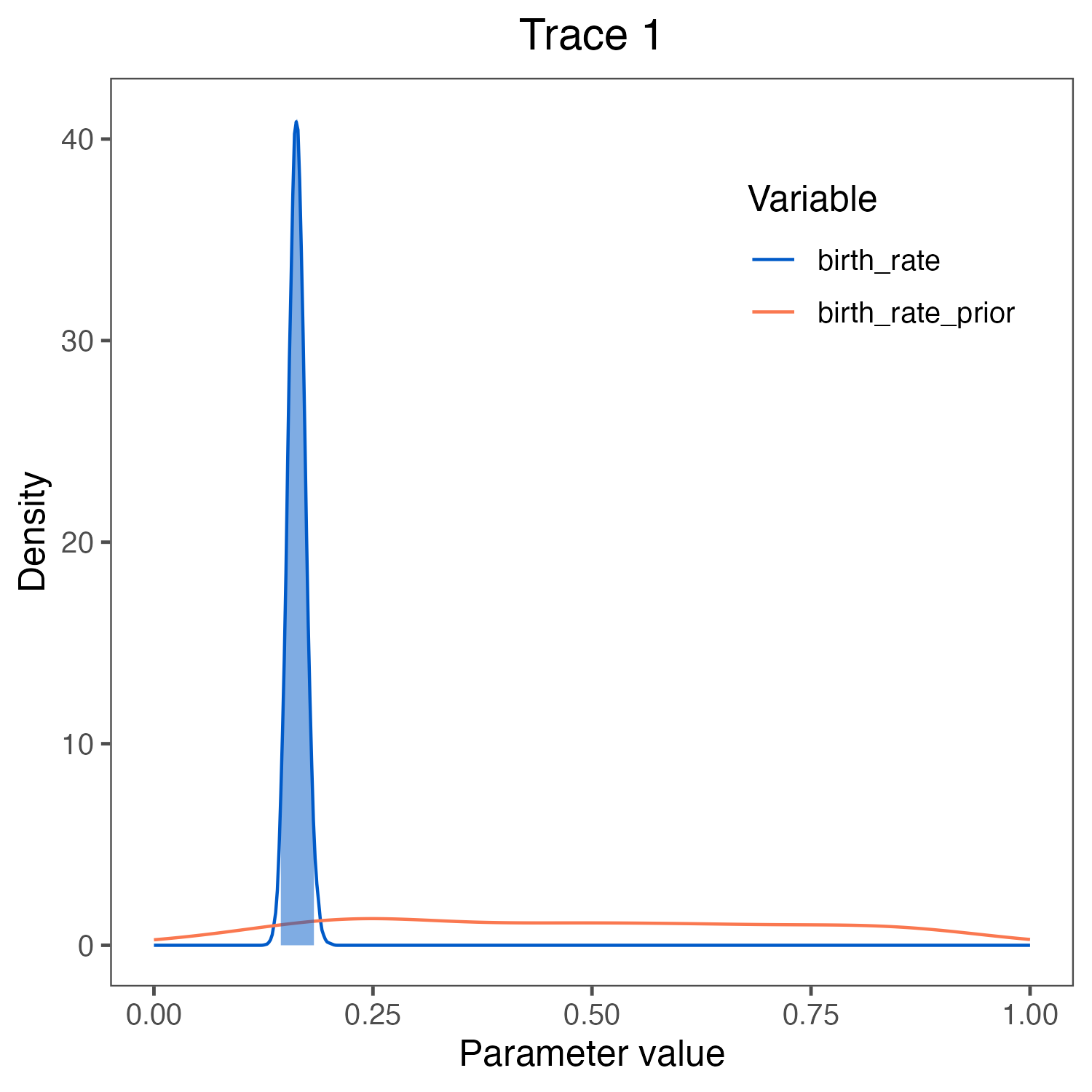
birth_rate visualized in
RevGadgets (Tribble et al. 2022).
We used the script plot_Yule_rates.R.
The prior (red curve) shows the lognormal distribution that we chose as the prior distribution.Estimating the marginal likelihood of the model
With a fully specified model, we can set up the powerPosterior()
analysis to create a file of ‘powers’ and likelihoods from which we can
estimate the marginal likelihood using stepping-stone or path sampling.
This method computes a vector of powers from a beta distribution, then
executes an MCMC run for each power step while raising the likelihood to
that power. In this implementation, the vector of powers starts with 1,
sampling the likelihood close to the posterior and incrementally
sampling closer and closer to the prior as the power decreases. For more
information on marginal likelihood estimation please read the
Bayesian Model Selection Tutorial or see Höhna et al. (2021).
First, we create the variable containing the power posterior. This
requires us to provide a model and vector of moves, as well as an output
file name. The cats argument sets the number of power steps.
pow_p = powerPosterior(mymodel, moves, monitors, "output/Yule_powp.out", cats=127, sampleFreq=10)
We can start the power posterior by first burning in the chain and and discarding the first 10000 states.
pow_p.burnin(generations=10000,tuningInterval=200)
Now execute the run with the .run() function:
pow_p.run(generations=10000)
Once the power posteriors have been saved to file, create a stepping-stone sampler. This function can read any file of power posteriors and compute the marginal likelihood using stepping-stone sampling.
ss = steppingStoneSampler(file="output/Yule_powp.out", powerColumnName="power", likelihoodColumnName="likelihood")
Compute the marginal likelihood under stepping-stone sampling using the
member function marginal() of the ss variable and record the value
in .
write("Stepping stone marginal likelihood:\t", ss.marginal() )
Path sampling is an alternative to stepping-stone sampling and also takes the same power posteriors as input.
ps = pathSampler(file="output/Yule_powp.out", powerColumnName="power", likelihoodColumnName="likelihood")
Compute the marginal likelihood under stepping-stone sampling using the
member function marginal() of the ps variable and record the value
in .
write("Path-sampling marginal likelihood:\t", ps.marginal() )
⇨ The Rev file for performing this analysis: ml_Yule.Rev.
Exercise 2
- Compute the marginal likelihood under the Yule model.
- Enter the estimate in the table below.
| Model | Path-Sampling | Stepping-Stone-Sampling |
|---|---|---|
| Marginal likelihood Yule ($M_0$) | ||
| Marginal likelihood birth-death ($M_1$) | ||
| Supported model? |
Birth-Death Process
The pure-birth model does not account for extinction, thus it assumes that every lineage at the start of the process will have sampled descendants at time 0. This assumption is fairly unrealistic for most phylogenetic datasets on a macroevolutionary time scale since the fossil record provides evidence of extinct lineages. Kendall (1948) described a more general branching process model to account for lineage extinction called the birth-death process. Under this model, at any instant in time, every lineage has the same rate of speciation $\lambda$ and the same rate of extinction $\mu$. This is the constant-rate birth-death process, which considers the rates constant over time and over the tree (Nee et al. 1994; Höhna 2015).
Yang and Rannala (1997) derived the probability of time trees under an extension of the birth-death model that accounts for incomplete sampling of the tips () (see also Stadler (2009), Höhna et al. (2011) and Höhna (2014)). Under this model, the parameter $\rho$ accounts for the probability of sampling in the present time, and because it is a probability, this parameter can only take values between 0 and 1. For more information on incomplete taxon sampling, see Diversification Rate Estimation with Missing Taxa tutorial.
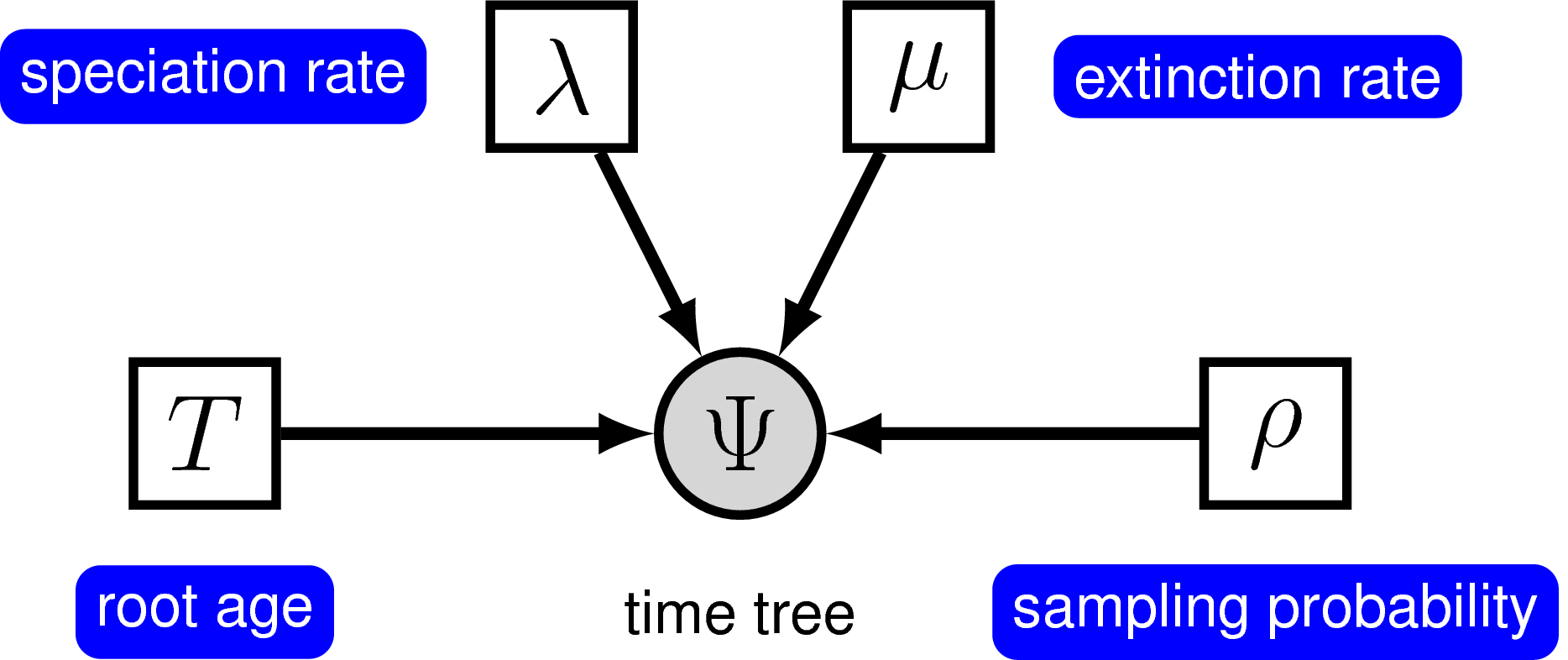
In principle, we can specify a model with prior distributions on speciation and extinction rates directly. One possibility is to specify an exponential, lognormal, or gamma distribution as the prior on either rate parameter. However, it is more common to specify prior distributions on a transformation of the speciation and extinction rate because, for example, we want to enforce that the speciation rate is always larger than the extinction rate.

In the following subsections we will only provide the key command that
are different for the constant-rate birth-death process. All other
commands will be the same as in the previous exercise. You should copy
the mcmc_Yule.Rev script and modify it accordingly. Don’t forget to
rename the filenames of the monitors to avoid overwriting of your
previous results!
Birth rate and death rate
Previously we assumed a uniform prior on the birth rate to signal that we have little information. The only information we use is that the rates are positive and smaller than 10 events per lineage per million years. We will apply this same prior distribution now for our birth-death model for both the birth and death rate.
birth_rate ~ dnUniform(0,100.0)
death_rate ~ dnUniform(0,100.0)
As before we will apply scaling moves on both parameters.
moves.append( mvScale(birth_rate,lambda=1.0,tune=true,weight=3.0) )
moves.append( mvScale(death_rate,lambda=1.0,tune=true,weight=3.0) )
The birth and death rates are likely to be correlated, i.e., we will get
better MCMC mixing if you jointly update both the birth and death rates.
Joint updates can be done with our mvUpDownScale move.
up_down_scale = mvUpDownScale(weight=3.0)
up_down_scale.addVariable( birth_rate, up=TRUE )
up_down_scale.addVariable( death_rate, up=TRUE )
moves.append( up_down_scale )
Diversification and turnover
The birth and death rates are our stochastic parameters and intrinsic
parameters. However, often we are also interested in the diversification and
relative extinction rate (or sometimes called turnover rate), which are simple
transformations of our birth and death rates. Thus, we create some deterministic
variables called diversification and rel_extinction.
diversification := birth_rate - death_rate
rel_extinction  := death_rate / birth_rate
All other parameters, such as the sampling probability and the root age are kept the same as in the analysis above.
The time tree
Initialize the stochastic node representing the time tree. The main difference now is that we provide a stochastic parameter for the extinction rate $\mu$.
timetree ~ dnBDP(lambda=birth_rate, mu=death_rate, rho=rho, rootAge=root_time, samplingStrategy="uniform", condition="survival", taxa=taxa)
⇨ The Rev file for performing this analysis: mcmc_BD.Rev
Exercise 3
- Run an MCMC simulation to compute the posterior distribution of the diversification and turnover rate.
- Look at the parameter estimates in
Tracer. What can you say about the diversification, turnover, speciation and extinction rates? How high is the extinction rate compared with the speciation rate? - Compute the marginal likelihood under the BD model. Which model is supported by the data?
- Enter the estimate in the table above.
- Can you modify the script to use a prior on the birth drawn from a
lognormal distribution and relative death rate drawn from a beta
distribution so that the extinction rate is equal to the birth rate
times the relative death rate?
- Do the parameter estimates change?
- What about the marginal likelihood estimates?
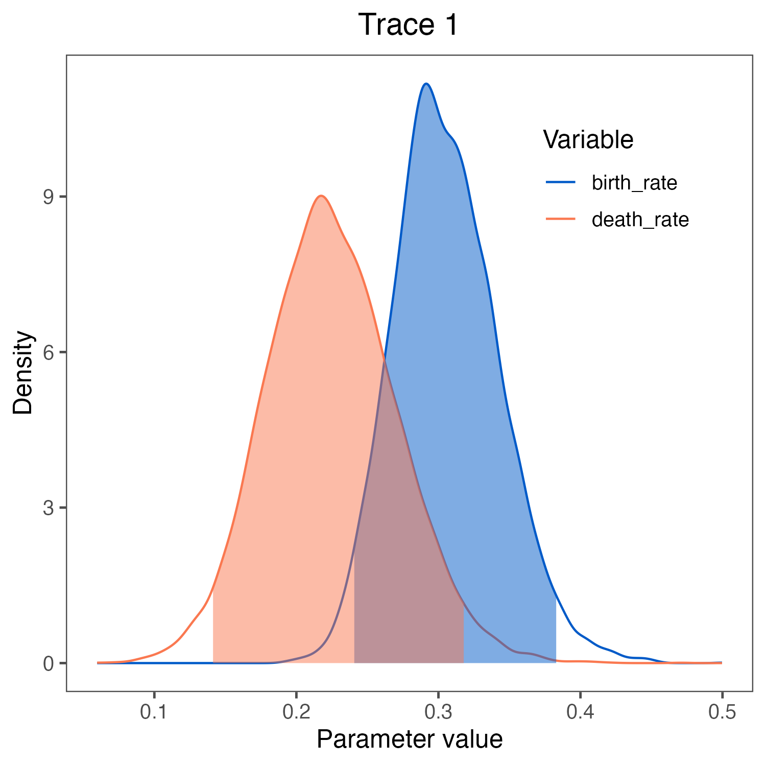
birth_rate and death_rate visualized in RevGadgets (Tribble et al. 2022).
We used the script plot_BD_rates.R.Click below to begin the next exercise!
- Aldous D.J. 2001. Stochastic models and descriptive statistics for phylogenetic trees, from Yule to today. Statistical Science.:23–34.
- Höhna S. 2014. Likelihood Inference of Non-Constant Diversification Rates with Incomplete Taxon Sampling. PLoS One. 9:e84184. 10.1371/journal.pone.0084184
- Höhna S. 2015. The time-dependent reconstructed evolutionary process with a key-role for mass-extinction events. Journal of Theoretical Biology. 380:321–331. http://dx.doi.org/10.1016/j.jtbi.2015.06.005
- Höhna S., Heath T.A., Boussau B., Landis M.J., Ronquist F., Huelsenbeck J.P. 2014. Probabilistic Graphical Model Representation in Phylogenetics. Systematic Biology. 63:753–771. 10.1093/sysbio/syu039
- Höhna S., Landis M.J., Huelsenbeck J.P. 2021. Parallel power posterior analyses for fast computation of marginal likelihoods in phylogenetics. PeerJ. 9:e12438.
- Höhna S., Stadler T., Ronquist F., Britton T. 2011. Inferring speciation and extinction rates under different species sampling schemes. Molecular Biology and Evolution. 28:2577–2589.
- Kendall D.G. 1948. On the Generalized "Birth-and-Death" Process. The Annals of Mathematical Statistics. 19:1–15. 10.1214/aoms/1177730285
- Magnuson-Ford K., Otto S.P. 2012. Linking the Investigations of Character Evolution and Species Diversification. The American Naturalist. 180:225–245. 10.1086/666649
- Nee S., May R.M., Harvey P.H. 1994. The Reconstructed Evolutionary Process. Philosophical Transactions: Biological Sciences. 344:305–311. 10.1098/rstb.1994.0068
- Stadler T. 2009. On incomplete sampling under birth-death models and connections to the sampling-based coalescent. Journal of Theoretical Biology. 261:58–66. 10.1016/j.jtbi.2009.07.018
- Thompson E.A. 1975. Human evolutionary trees. Cambridge University Press Cambridge.
- Tribble C.M., Freyman W.A., Landis M.J., Lim J.Y., Barido-Sottani J., Kopperud B.T., Höhna S., May M.R. 2022. RevGadgets: An R package for visualizing Bayesian phylogenetic analyses from RevBayes. Methods in Ecology and Evolution. 13:314–323. https://doi.org/10.1111/2041-210X.13750
- Yang Z., Rannala B. 1997. Bayesian phylogenetic inference using DNA sequences: a Markov Chain Monte Carlo Method. Molecular Biology and Evolution. 14:717–724. 10.1093/oxfordjournals.molbev.a025811
- Yule G.U. 1925. A mathematical theory of evolution, based on the conclusions of Dr. JC Willis, FRS. Philosophical Transactions of the Royal Society of London. Series B, Containing Papers of a Biological Character. 213:21–87.