Overview: Diversification Rate Estimation
Stochastic branching models allow for inference of speciation and extinction rates. In these tutorials we focus on the different types of macroevolutionary models to study diversification processes and thus the diversification-rate parameters themselves.
Types of Hypotheses for Estimating Diversification Rates
Macroevolutionary diversification rate estimation focuses on different key hypothesis, which may include: adaptive radiation, diversity-dependent and character diversification, key innovations, and mass extinction. We classify these hypotheses primarily into questions whether diversification rates vary through time, and if so, whether some external, global factor has driven diversification rate changes, or if diversification rates vary among lineages, and if so, whether some species specific factor is correlated with the diversification rates.
Below, we describe each of the fundamental questions regarding diversification rates.
(1) Constant diversification-rate estimation
What is the global rate of diversification in my phylogeny? The most basic models estimate parameters of the birth-death process (i.e., rates of speciation and extinction, or composite parameters such as net-diversification and relative-extinction rates) under the assumption that rates have remained constant across lineages and through time. This is the most basic example and should be treated as a primer and introduction into the topic.
For more information, we recommend the Simple Diversification Rate Estimation.
(2) Diversification rate variation through time
Is there diversification rate variation through time in my phylogeny? There are several reasons why diversification rates for the entire study group can vary through time, for example: adaptive radiation, diversity dependence and mass-extinction events. We can detect a signal any of these causes by detecting diversification rate variation through time.
The different tutorials references below cover different scenarios for diversification rate variation through time. The common theme of these studies is that the diversification process is tree-wide, that is, all lineages of the study group have the exact same rates at a given time.
(2a) Detecting diversification rate variation through time
In RevBayes we use an episodic birth-death model to study diversification rate variation through time. That is, we assume that diversification rates are constant within an epoch but may shift between episodes (Stadler (2011), Höhna (2015)). Then, we are estimating the diversification rates for each episode, and thus diversification rate variation through time.
You can find examples and more information in the Episodic Diversification Rate Estimation.
(2b) Detecting the impact of mass-extinction events on diversification
Another question in this category asks whether our study tree was impacted by a mass-extinction event (where a large fraction of the standing species diversity is suddenly lost, e.g., Höhna (2015), May et al. (2016), Magee and Höhna (2021)). That is, we infer and test for the impact of instantaneous mass extinction events where each species alive at the given time has a probability of survival of the event.
You can find examples and more information in the Mass Extinction Estimation.
(2c) Diversification-rate correlation to environmental (e.g., abiotic) factors
Are diversification rates correlated with some abiotic (e.g., environmental) variable in my phylogeny? If we have found evidence in the previous section that diversification rates vary through time, then we can start asking the question whether these changes in diversification rates are driven by some abiotic (e.g., environmental) factors. For example, we can ask whether changes in diversification rates are correlated with environmental factors, such as environmental CO2 or temperature (Condamine et al. 2013; Condamine et al. 2018; Palazzesi et al. 2022).
You can find examples and more information in the Environmental-dependent Speciation & Extinction Rates.
(3) Diversification-rate variation across branches estimation
Is there diversification rate variation among lineages in my phylogeny? There are several reasons why diversification rates can vary among lineages primarily due to species specific factors (intrinsic and extrinsic), for example, key innovations. First, we can try to detect a signal of rate variation among lineages, and then we can test if their are variables that are associated with this among lineage rate variation. The different tutorials references below cover different scenarios for diversification rate variation among lineages.
(3a) Detecting diversification-rate variation across branches estimation
Is there evidence that diversification rates have varied across the branches of my phylogeny? Have there been significant diversification-rate shifts along branches in my phylogeny, and if so, how many shifts, what magnitude of rate-shifts and along which branches? Similarly, one may ask what are the branch-specific diversification rates?
You can study diversification rate variation among lineages using our birth-death-shift process (Höhna et al. 2019). Examples and more information is provided in the Branch-Specific Diversification Rate Estimation.
(3b) Character-dependent diversification-rate estimation
If we have found that there is rate variation among lineage, then we could ask if diversification rates correlated with some biotic (e.g., morphological) variable. This can be addressed by using character-dependent birth-death models (often also called state-dependent speciation and extinction models; SSE models). Character-dependent diversification-rate models aim to identify overall correlations between diversification rates and organismal features (binary and multi-state discrete morphological traits, continuous morphological traits, geographic range, etc.). For example, one can hypothesize that a binary character, say if an organism is herbivorous/carnivorous or self-compatible/self-incompatible, impact the diversification rates. Then, if the organism is in state 0 (e.g., is herbivorous) it has a lower (or higher) diversification rate than if the organism is in state 1 (e.g., carnivorous) (Maddison et al. 2007).
You can find examples and more information in
- Background on state-dependent diversification rate estimation
- State-dependent diversification with BiSSE and MuSSE tutorial
- State-dependent diversification with HiSSE tutorial
- State-dependent diversification with the ClaSSE model tutorial
- Chromosome Evolution tutorial
(4) General Extension to Diversification Rate Estimation
There exist some general considerations, assumptions and extensions that apply to most/all diversification rate models. We provide a few general topics.
(4a) Incomplete taxon sampling
For most study groups, we do not have all extant taxa sampled. It is important that we properly model incomplete taxon sampling because otherwise our parameter estimates are biased (Höhna et al. 2011; Höhna 2014; Palazzesi et al. 2022). You can find examples and more information in the Diversification Rate Estimation with Missing Taxa.
(4b) Conditions of the Birth-Death Process
As any statistical model, the birth-death process includes several assumptions/conditions. Primarily, we condition the process if we only consider study groups that (a) survived until the present, (b) left exactly $N$ extant taxa, or (c) no restrictions. The conditions become a bit more involved if phylogenies with fossils are considered. You can find more discussion and examples in the Conditions of the Birth-Death Process section below.
Diversification Rate Models
We begin this section with a general introduction to the stochastic birth-death branching process that underlies inference of diversification rates in RevBayes. This primer will provide some details on the relevant theory of stochastic-branching process models. We appreciate that some readers may want to skip this somewhat technical primer; however, we believe that a better understanding of the relevant theory provides a foundation for performing better inferences. We then discuss a variety of specific birth-death models, but emphasize that these examples represent only a tiny fraction of the possible diversification-rate models that can be specified in RevBayes.
The birth-death branching process
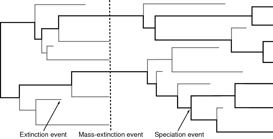
Our approach is based on the reconstructed evolutionary process described by (Nee et al. 1994); a birth-death process in which only sampled, extant lineages are observed. Let $N(t)$ denote the number of species at time $t$. Assume the process starts at time $t_1$ (the ‘crown’ age of the most recent common ancestor of the study group, $t_\text{MRCA}$) when there are two species. Thus, the process is initiated with two species, $N(t_1) = 2$. We condition the process on sampling at least one descendant from each of these initial two lineages; otherwise $t_1$ would not correspond to the $t_\text{MRCA}$ of our study group. Each lineage evolves independently of all other lineages, giving rise to exactly one new lineage with rate $b(t)$ and losing one existing lineage with rate $d(t)$ ( and ). Note that although each lineage evolves independently, all lineages share both a common (tree-wide) speciation rate $b(t)$ and a common extinction rate $d(t)$ (Nee et al. 1994; Höhna 2015). Additionally, at certain times, $t_{\mathbb{M}}$, a mass-extinction event occurs and each species existing at that time has the same probability, $\rho$, of survival. Finally, all extinct lineages are pruned and only the reconstructed tree remains ().
To condition the probability of observing the branching times on the survival of both lineages that descend from the root, we divide by $P(N(T) > 0 | N(0) = 1)^2$. Then, the probability density of the branching times, $\mathbb{T}$, becomes
\[\begin{aligned} P(\mathbb{T}) = \frac{\overbrace{P(N(T) = 1 \mid N(0) = 1)^2}^{\text{both initial lineages have one descendant}}}{ \underbrace{P(N(T) > 0 \mid N(0) = 1)^2}_{\text{both initial lineages survive}} } \times \prod_{i=2}^{n-1} \overbrace{i \times b(t_i)}^{\text{speciation rate}} \times \overbrace{P(N(T) = 1 \mid N(t_i) = 1)}^\text{lineage has one descendant}, \end{aligned}\]and the probability density of the reconstructed tree (topology and branching times) is then
\[\begin{aligned} P(\Psi) = \; & \frac{2^{n-1}}{n!(n-1)!} \times \left( \frac{P(N(T) = 1 \mid N(0) = 1)}{P(N(T) > 0 \mid N(0) = 1)} \right)^2 \nonumber\\ \; & \times \prod_{i=2}^{n-1} i \times b(t_i) \times P(N(T) = 1 \mid N(t_i) = 1) \label{eq:tree_probability} \end{aligned}\]We can expand Equation ([eq:tree_probability]) by substituting $P(N(T) > 0 \mid N(t) =1)^2 \exp(r(t,T))$ for $P(N(T) = 1 \mid N(t) = 1)$, where $r(u,v) = \int^v_u d(t)-b(t)dt$; the above equation becomes
\[\begin{aligned} P(\Psi) = \; & \frac{2^{n-1}}{n!(n-1)!} \times \left( \frac{P(N(T) > 0 \mid N(0) =1 )^2 \exp(r(0,T))}{P(N(T) > 0 \mid N(0) = 1)} \right)^2 \nonumber\\ \; & \times \prod_{i=2}^{n-1} i \times b(t_i) \times P(N(T) > 0 \mid N(t_i) = 1)^2 \exp(r(t_i,T)) \nonumber\\ = \; & \frac{2^{n-1}}{n!} \times \Big(P(N(T) > 0 \mid N(0) =1 ) \exp(r(0,T))\Big)^2 \nonumber\\ \; & \times \prod_{i=2}^{n-1} b(t_i) \times P(N(T) > 0 \mid N(t_i) = 1)^2 \exp(r(t_i,T)). \label{eq:tree_probability_substitution} \end{aligned}\]For a detailed description of this substitution, see Höhna (2015). Additional information regarding the underlying birth-death process can be found in Thompson (1975) [Equation 3.4.6] and Nee et al. (1994) for constant rates and Höhna (2013), Höhna (2014), Höhna (2015) for arbitrary rate functions.
To compute the equation above we need to know the rate function, $r(t,s) = \int_t^s d(x)-b(x) dx$, and the probability of survival, $P(N(T)!>!0|N(t)!=!1)$. Yule (1925) and later Kendall (1948) derived the probability that a process survives ($N(T) > 0$) and the probability of obtaining exactly $n$ species at time $T$ ($N(T) = n$) when the process started at time $t$ with one species. Kendall’s results were summarized in Equation (3) and Equation (24) in Nee et al. (1994)
\[\begin{aligned} P(N(T)\!>\!0|N(t)\!=\!1) & = & \left(1+\int\limits_t^{T} \bigg(\mu(s) \exp(r(t,s))\bigg) ds\right)^{-1} \label{eq:survival} \\ \nonumber \\ P(N(T)\!=\!n|N(t)\!=\!1) & = & (1-P(N(T)\!>\!0|N(t)\!=\!1)\exp(r(t,T)))^{n-1} \nonumber\\ & & \times P(N(T)\!>\!0|N(t)\!=\!1)^2 \exp(r(t,T)) \label{eq:N} %\\ %P(N(T)\!=\!1|N(t)\!=\!1) & = & P(N(T)\!>\!0|N(t)\!=\!1)^2 \exp(r(t,T)) \label{eq:1} \end{aligned}\]An overview for different diversification models is given in Höhna (2015).
Phylogenetic trees as observations
The branching processes used here describe probability distributions on phylogenetic trees. This probability distribution can be used to infer diversification rates given an “observed” phylogenetic tree. In reality we never observe a phylogenetic tree itself. Instead, phylogenetic trees themselves are estimated from actual observations, such as DNA sequences. These phylogenetic tree estimates, especially the divergence times, can have considerable uncertainty associated with them. Thus, the correct approach for estimating diversification rates is to include the uncertainty in the phylogeny by, for example, jointly estimating the phylogeny and diversification rates. For the simplicity of the following tutorials, we take a shortcut and assume that we know the phylogeny without error. For publication quality analysis you should always estimate the diversification rates jointly with the phylogeny and divergence times.
Conditions of the Birth-Death Process
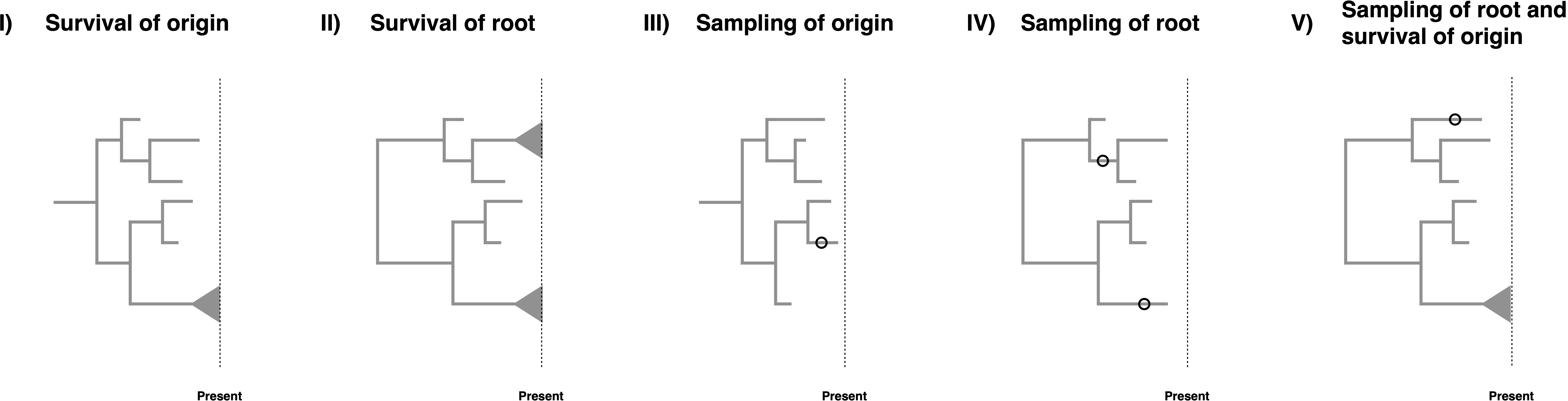
Birth-death models are often conditioned on specific events, see (Stadler 2013), (Höhna 2015) and (Magee and Höhna 2021) for some discussion on the topic. However, when there are non-contemporaneous samples in the dataset which may be ancestral to other samples, conditioning becomes somewhat complex. The key issues for conditioning are whether it is assumed that the process starts at the root or the origin, and whether the descending lineage(s) is (are) assumed to leave any sampled descendant or specifically to have a descendant sampled at the present day. Consideration of these possibilities leads to five possible conditions, though conditioning is not strictly required.
- Survival of the origin: We condition the process on survival of one lineage, i.e., at least on descendant of the lineage starting at the origin was sampled at the present. This condition represent a case when we have fossils and extant taxa and do not know if the fossils are stem fossils of the entire clade. The condition is obtained by computing $1-E(t_{or})$ with $\phi(t)=0$.
- Survival of the root: We condition the process on survival of both lineages, i.e., at least one descendant of each lineage starting at the root was sampled at the present. This is the case for most macroevolutionary analyses without any fossils or if the fossils are known to belong within the crown group of the extant taxa. The condition is obtained by computing $(1-E(t_{MRCA}))^2$ with $\phi(t)=0$.
- Sampling of origin: We condition the process to have at least one sample being a descendant of the origin. This is simply a minimal condition that at least something was observed/sampled. This condition represents the case if we would also consider complete extinct clades. The condition is obtained by computing $1-E(t_{or})$.
- Sampling of the root: We condition the process to require that both lineages starting at the root are sampled. In this case, all taxa might be extinct but the root age is known or inferred as a parameter of the model. The condition is obtained by computing $(1-E(t_{MRCA}))^2$.
- Sampling of the root and survival of the origin: We condition the process on sampling of both descendant lineages of the root and at least one sample at the present. In this case, we condition on this specific root age but one of the descendant lineages of the root might have gone extinct while the other descendant lineage from the root must have survived. The condition is obtained by computing $(1-E_{\phi(t)=0}(t_{MRCA}))(1-E_{\phi(t)\neq 0}(t_{MRCA}))$.
For macroevolutionary analyses of diversification rates, condition (I) is the most adequate if we have both extinct and extant taxa, condition (II) if we have only extant taxa, and condition (III) if we have only extinct taxa. For phylodynamic applications, if it can safely be assumed that there are no sampled ancestors prior to the first observed infection (which will always be true if $r(t) = 1$), condition (IV) may be used, otherwise only condition (III) is applicable. Conditioning on survival as in (I), (II), or (V) requires $\Phi_0 > 0$, and so is primarily of interest in macroevolutionary applications. Of these conditions, (II) is the strictest and requires prior knowledge that the MRCA of the extant samples is the MRCA of all samples. Condition (V) is less restrictive, requiring only that none of the fossils could be sampled ancestors prior to the first observed speciation event, which would apply if all fossils are within the crown group. We could additionally condition on the number of extant taxa $N$, as suggest by (Gernhard 2008), although there is, as of today and to our knowledge, no solution known to condition on the number of extinct taxa.
- Condamine F.L., Rolland J., Morlon H. 2013. Macroevolutionary perspectives to environmental change. Ecology Letters. 10.1111/ele.12062
- Condamine F.L., Rolland J., Höhna S., Sperling F.A.H., Sanmartín I. 2018. Testing the role of the Red Queen and Court Jester as drivers of the macroevolution of Apollo butterflies. Systematic Biology. 67:940–964.
- Gernhard T. 2008. The conditioned reconstructed process. Journal of Theoretical Biology. 253:769–778. 10.1016/j.jtbi.2008.04.005
- Höhna S. 2013. Fast simulation of reconstructed phylogenies under global time-dependent birth-death processes. Bioinformatics. 29:1367–1374. 10.1093/bioinformatics/btt153
- Höhna S. 2014. Likelihood Inference of Non-Constant Diversification Rates with Incomplete Taxon Sampling. PLoS One. 9:e84184. 10.1371/journal.pone.0084184
- Höhna S. 2015. The time-dependent reconstructed evolutionary process with a key-role for mass-extinction events. Journal of Theoretical Biology. 380:321–331. http://dx.doi.org/10.1016/j.jtbi.2015.06.005
- Höhna S., Freyman W.A., Nolen Z., Huelsenbeck J.P., May M.R., Moore B.R. 2019. A Bayesian Approach for Estimating Branch-Specific Speciation and Extinction Rates. bioRxiv. 10.1101/555805
- Höhna S., Stadler T., Ronquist F., Britton T. 2011. Inferring speciation and extinction rates under different species sampling schemes. Molecular Biology and Evolution. 28:2577–2589.
- Kendall D.G. 1948. On the Generalized "Birth-and-Death" Process. The Annals of Mathematical Statistics. 19:1–15. 10.1214/aoms/1177730285
- Maddison W.P., Midford P.E., Otto S.P. 2007. Estimating a binary character’s effect on speciation and extinction. Systematic Biology. 56:701. 10.1080/10635150701607033
- Magee A.F., Höhna S. 2021. Impact of K-Pg Mass Extinction Event on Crocodylomorpha Inferred from Phylogeny of Extinct and Extant Taxa. bioRxiv.:426715. 10.1101/426715
- May M.R., Höhna S., Moore B.R. 2016. A Bayesian Approach for Detecting the Impact of Mass-Extinction Events on Molecular Phylogenies When Rates of Lineage Diversification May Vary. Methods in Ecology and Evolution. 7:947–959. 10.1111/2041-210X.12563
- Nee S., May R.M., Harvey P.H. 1994. The Reconstructed Evolutionary Process. Philosophical Transactions: Biological Sciences. 344:305–311. 10.1098/rstb.1994.0068
- Palazzesi L., Hidalgo O., Barreda V.D., Forest F., Höhna S. 2022. The rise of grasslands is linked to atmospheric CO\textsubscript2 decline in the late Paleogene. Nature Communications. 13:293.
- Stadler T. 2011. Mammalian phylogeny reveals recent diversification rate shifts. Proceedings of the National Academy of Sciences. 108:6187–6192. 10.1073/pnas.1016876108
- Stadler T. 2013. How can we improve accuracy of macroevolutionary rate estimates? Systematic Biology. 62:321–329.
- Thompson E.A. 1975. Human evolutionary trees. Cambridge University Press Cambridge.
- Yule G.U. 1925. A mathematical theory of evolution, based on the conclusions of Dr. JC Willis, FRS. Philosophical Transactions of the Royal Society of London. Series B, Containing Papers of a Biological Character. 213:21–87.