State-dependent diversification with BiSSE and MuSSE

Inference using the binary/multiple state-dependent speciation and extinction (BiSSE/MuSSE) branching process

Sebastian Höhna, Will Freyman, and Emma Goldberg

Last modified on March 11, 2022

Introduction

This tutorial describes how to specify character state-dependent branching process models in RevBayes (Höhna et al. 2016). For more details on the theory behind these models, please see the introductory page: Background on state-dependent diversification rate estimation.

This tutorial will explain how to fit the BiSSE and MuSSE models to data using Markov chain Monte Carlo (MCMC). RevBayes is a powerful tool for SSE analyses: to specify HiSSE model, please see State-dependent diversification with HiSSE, for the ClaSSE model, please see State-dependent diversification with the ClaSSE model and for ChromoSSE please see Chromosome Evolution.

Getting Set Up

We provide the data files which we will use in this tutorial:

primates_tree.nex: Dated primate phylogeny including 233 out of 367 species. This tree is from Magnuson-Ford and Otto (2012), who took it from Vos and Mooers (2006) and then randomly resolved the polytomies using the method of Kuhn et al. (2011).
primates_activity_period.nex: A file with the coded character states for primate species activity time. This character has just two states: 0 = diurnal and 1 = nocturnal.
primates_solitariness.nex: A file with the coded character states for primate species social system type. This character has just two states: 0 = group living and 1 = solitary.
primates_mating_system.nex: A file with the coded character states for primate species mating-system type. This character has four states: 0 = monogamy, 1 = polygyny, 2 = polygynandry, and 3 = polyandry.

Create a new directory on your computer called RB_bisse_tutorial.

Within the RB_bisse_tutorial directory, create a subdirectory called data. Then, download the provided files and place them in the data folder.

Estimating State-Dependent Speciation and Extinction under the BiSSE Model

Now let’s start to analyze an example in RevBayes using the BiSSE model. In RevBayes, it’s called CDBDP, meaning character dependent birth-death process.

Navigate to the RB_bisse_tutorial directory and execute the rb binary. One option for doing this is to move the rb executable to the RB_bisse_tutorial directory.

Alternatively, if you are on a Unix system, and have added RevBayes to your path, you simply have to type rb in your Terminal to run the program.

For this tutorial, we will specify a BiSSE model that allows for speciation and extinction to be correlated with a particular life-history trait: the timing of activity during the day. If you open the file primates_activity_period.nex in your text editor, you will see that several species like the mantled howler monkey (Alouatta palliata) have the state 0, indicating that they are diurnal. Whereas other nocturnal species, like the aye-aye (Daubentonia madagascariensis) are coded with 1. We may have an a priori hypothesis that diurnal species have higher rates of speciation and by estimating the rates of lineages associated with that trait will allow us to explore this hypothesis.

Once you execute RevBayes, you will be in the console. The rest of this tutorial will proceed using the interactive console.

Read in the Data

For this tutorial, we are assuming that the tree is “observed” and considered data. Thus, we will read in the dated phylogeny first.

observed_phylogeny <- readTrees("data/primates_tree.nex")[1]

Next, we will read in the observed character states for primate activity period.

data <- readCharacterData("data/primates_activity_period.nex")

It will be convenient to get the number of sampled species num_taxa from the tree:

num_taxa <- observed_phylogeny.ntips()

Additionally, we initialize a variable for our vector of moves and monitors.

moves    = VectorMoves()
monitors = VectorMonitors()

Finally, create a helper variable that specifies the number of states that the observed character has:

NUM_STATES = 2

Using this variable allows us to easily change our script and use a different character with a different number of states, essentially changing our model from BiSSE (Maddison et al. 2007) to one that allows for more than 2 states–i.e., the MuSSE model (FitzJohn 2012).

Specify the Model

The basic idea behind the model in this example is that speciation and extinction rates are dependent on a binary character, and the character transitions between its two possible states (Maddison et al. 2007).

Priors on the Rates

We start by specifying prior distributions on the diversification rates. Here, we will assume an identical prior distribution on each of the speciation and extinction rates. Furthermore, we will use a log-uniform distribution as the prior distribution on each speciation and extinction rate (i.e., a uniform distribution on the log of the rates).

Now we can specify our character-specific speciation and extinction rate parameters. Because we will use the same prior for each rate, it’s easy to specify them all in a for-loop. We will use a log-uniform distribution as a prior on the speciation and extinction rates. The loop also allows us to apply moves to each of the rates we are estimating and create a vector of deterministic nodes representing the rate of diversification ($\lambda - \mu$) associated with each character state.

for (i in 1:NUM_STATES) {

     ### Create a loguniform distributed variable for the diversification rate
    speciation[i] ~ dnLoguniform( 1E-6, 1E2)
    moves.append( mvScale(speciation[i],lambda=0.20,tune=true,weight=3.0) )

    ### Create a loguniform distributed variable for the turnover rate
    extinction[i] ~ dnLoguniform( 1E-6, 1E2)
    moves.append( mvScale(extinction[i],lambda=0.20,tune=true,weight=3.0) )


    diversification[i] := speciation[i] - extinction[i]

}

The stochastic nodes representing the vector of speciation rates and vector of extinction rates have been instantiated. The software assumes that the rate in position [1] of each vector corresponds to the rate associated with diurnal 0 lineages and the rate at position [2] of each vector is the rate associated with nocturnal 1 lineages.

⇨ If RevBayes has trouble finding good starting values, then you can initialize the speciation and extinction rate as follows:

speciation[i].setValue( ln(367.0/2.0) / observed_phylogeny.rootAge() )
extinction[i].setValue( speciation/10.0 )

You can print the current values of the speciation rate vector to your screen:

speciation

[ 0.267, 0.160 ]

Of course, your screen output will be different from the values shown above since your stochastic nodes were initialized with different values drawn from the exponential prior.

Next we specify the transition rates between the states 0 and 1: $q_{01}$ and $q_{10}$. As a prior, we choose that each transition rate is drawn from an exponential distribution with a mean of 10 character state transitions over the entire tree. This is reasonable because we use this kind of model for traits that transition not-infrequently, and it leaves a fair bit of uncertainty. Note that we will actually use a for-loop to instantiate the transition rates so that our script will also work for non-binary characters.

rate_pr := observed_phylogeny.treeLength() / 10
for ( i in 1:(NUM_STATES*(NUM_STATES-1)) ) {
    transition_rates[i] ~ dnExp(rate_pr)
    moves.append( mvScale(transition_rates[i],lambda=0.20,tune=true,weight=3.0) )
}

Here, rate[1] is the rate of transition from state 0 (diurnal) to state 1 (nocturnal), and rate[2] is the rate of going from nocturnal to diurnal.

Finally, we put the rates into a matrix, because this is what’s needed by the function for the state-dependent birth-death process.

rate_matrix := fnFreeK( transition_rates, rescaled=false)

Note that we do not “rescale” the rate matrix. Rate matrices for molecular evolution are rescaled to have an average rate of 1.0, but for this model we want estimates of the transition rates with the same time scale as the diversification rates.

Prior on the Root State

Create a variable for the root state frequencies. We are using a flat Dirichlet distribution as the prior on each state. There has been some discussion about this in (FitzJohn et al. 2009). You could also fix the prior probabilities for the root states to be equal (generally not recommended), or use empirical state frequencies.

root_state_freq ~ dnDirichlet( rep(1, NUM_STATES) )

Note that we use the rep() function which generates a vector of length NUM_STATES with each position in the vector set to 1. Using this function and the NUM_STATES variable allows us to easily use this Rev script as a template for a different analysis using a character with more than two states.

We will use a special move for objects that are drawn from a Dirichlet distribution:

append( mvDirichletSimplex(rate_category_prior,tune=true,weight=2) )

The Probability of Sampling an Extant Species

All birth-death processes are conditioned on the probability a taxon is sampled in the present. We can get an approximation for this parameter by calculating the proportion of sampled species in our analysis.

We know that we have sampled 233 out of 367 living described primate species. To account for this we can set the sampling probability as a constant node with a value of 233/367.

sampling <- num_taxa / 367

Root Age

The birth-death process also depends on time to the most-recent-common ancestor–i.e., the root. In this exercise we use a fixed tree and thus we know the age of the tree.

root_age <- T.rootAge()

The Time Tree

Now we have all of the parameters we need to specify the full character state-dependent birth-death model. We initialize the stochastic node representing the time tree and we create this node using the dnCDBDP() function.

timetree ~ dnCDBDP( rootAge           = root_age,
                    speciationRates   = speciation,
                    extinctionRates   = extinction,
                    Q                 = rate_matrix,
                    pi                = root_state_freq,
                    rho               = sampling )

Now, we will fix the BiSSE time-tree to the observed values from our data files. We use the standard .clamp() method to give the observed tree and branch times:

timetree.clamp( observed_phylogeny )

And then we use the .clampCharData() to set the observed states at the tips of the tree:

timetree.clampCharData( data )

Finally, we create a workspace object of our whole model. The model() function traverses all of the connections and finds all of the nodes we specified.

mymodel = model(timetree)

You can use the .graph() method of the model object to visualize the graphical model you have just constructed . This function writes the model DAG to a file that can be viewed using the program Graphviz ().

The probabilistic graphical model of the character-state-dependent diversification model. This image was generated by executing the `mymodel.graph("bisse.dot")` in RevBayes after specifying the full model DAG. Then, the resulting file can be opened in the program Graphviz.

Running an MCMC analysis

Specifying Monitors

For our MCMC analysis, we set up a vector of monitors to record the states of our Markov chain. The first monitor will model all numerical variables; we are particularly interested in the rates of speciation, extinction, and transition.

monitors.append( mnModel(filename="output/primates_BiSSE_activity_period.log", printgen=1) )

Optionally, we can sample ancestral states during the MCMC analysis. We need to add an additional monitor to record the state of each internal node in the tree. The file produced by this monitor can be summarized so that we can visualize the estimates of ancestral states.

monitors.append( mnJointConditionalAncestralState(tree=timetree,
                     cdbdp=timetree,  
                     type="Standard",
                     printgen=1,
                     withTips=true,
                     withStartStates=false,
                     filename="output/primates_BiSSE_activity_period_anc_states.log") )

Similarly, you may want to add a stochastic character map.

monitors.append( mnStochasticCharacterMap(cdbdp=timetree,
                       filename="output/primates_BiSSE_activity_period_stoch_map.log",
                       printgen=1) )

Then, we add a screen monitor showing some updates during the MCMC run.

monitors.append( mnScreen(printgen=10, speciation, extinction) )

Initializing and Running the MCMC Simulation

With a fully specified model, a set of monitors, and a set of moves, we can now set up the MCMC algorithm that will sample parameter values in proportion to their posterior probability. The mcmc() function will create our MCMC object:

mymcmc = mcmc(mymodel, monitors, moves, nruns=2, combine="mixed")

Now, run the MCMC:

mymcmc.run(generations=5000, tuningInterval=200)

Summarize Sampled Ancestral States

If we sampled ancestral states during the MCMC analysis, we can use the RevGadgets (Tribble et al. 2022) R package to plot the ancestral state reconstruction. First, though, we must summarize the sampled values in RevBayes.

To do this, we first have to read in the ancestral state log file. This uses a specific function called readAncestralStateTrace().

anc_states = readAncestralStateTrace("output/primates_BiSSE_activity_period_anc_states.log")

Now, we can write an annotated tree to a file. This function will write a tree with each node labeled with the maximum a posteriori (MAP) state and the posterior probabilities for each state.

anc_tree = ancestralStateTree(tree=T,
                  ancestral_state_trace_vector=anc_states,
                  include_start_states=false,
                  file="output/primates_BiSSE_anc_states_results.tree",
                  burnin=0,
                  summary_statistic="MAP",
                  site=1)

Similarly, we compute the maximum a posteriori (MAP) stochastic character map.

anc_state_trace = readAncestralStateTrace("output/primates_BiSSE_activity_period_stoch_map.log")
characterMapTree(observed_phylogeny,
                 anc_state_trace,
                 character_file="output/primates_BiSSE_activity_period_stoch_map_character.tree",
                 posterior_file="output/primates_BiSSE_activity_period_stoch_map_posterior.tree",
                 burnin=0.1,
                 reconstruction="marginal")

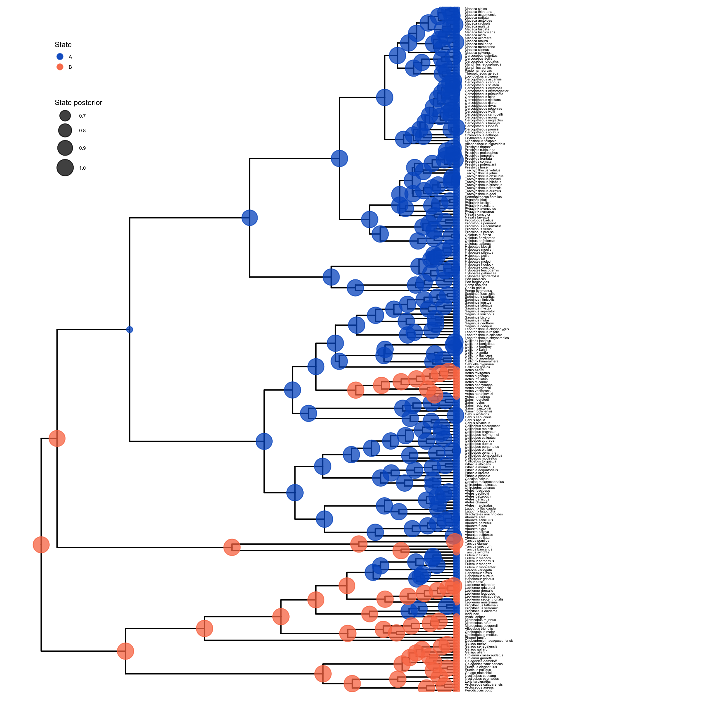
Visualize Estimated Ancestral States

To visualize the posterior probabilities of ancestral states, we will use the RevGadgets (Tribble et al. 2022) R package.

Open R.

RevGadgets requires the ggtree package (Yu et al. 2017). First, install the ggtree and RevGadgets packages:

install.packages("devtools")
library(devtools)
install_github("GuangchuangYu/ggtree")
install_github("revbayes/RevGadgets")

Run this code (or use the script plot_anc_states_BiSSE.R):

library(ggplot2)
library(RevGadgets)

# read in and process the ancestral states
bisse_file <- paste0("output/primates_BiSSE_activity_period_anc_states_results.tree")
p_anc <- processAncStates(bisse_file)

# plot the ancestral states
plot <- plotAncStatesMAP(p_anc,
        tree_layout = "rect",
        tip_labels_size = 1) +
        # modify legend location using ggplot2
        theme(legend.position = c(0.1,0.85),
              legend.key.size = unit(0.3, 'cm'), #change legend key size
              legend.title = element_text(size=6), #change legend title font size
              legend.text = element_text(size=4))

ggsave(paste0("BiSSE_anc_states_activity_period.png"),plot, width=8, height=8)

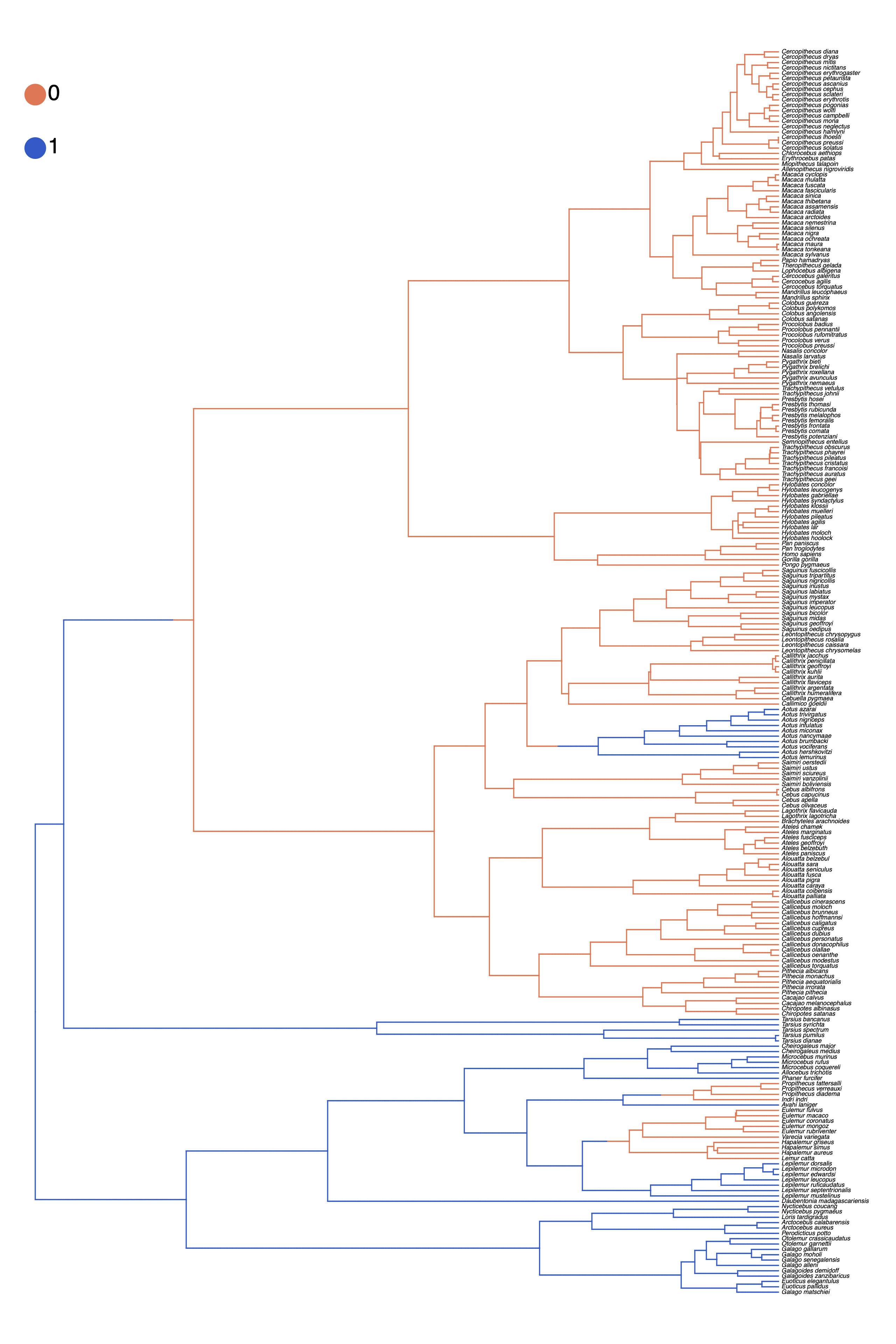
A visualization of the ancestral states estimated under the BiSSE model. We used the script `plot_anc_states_BiSSE.R`.

Next, we also want to plot the stochastic character map. Use the script plot_simmap_BiSSE.R.

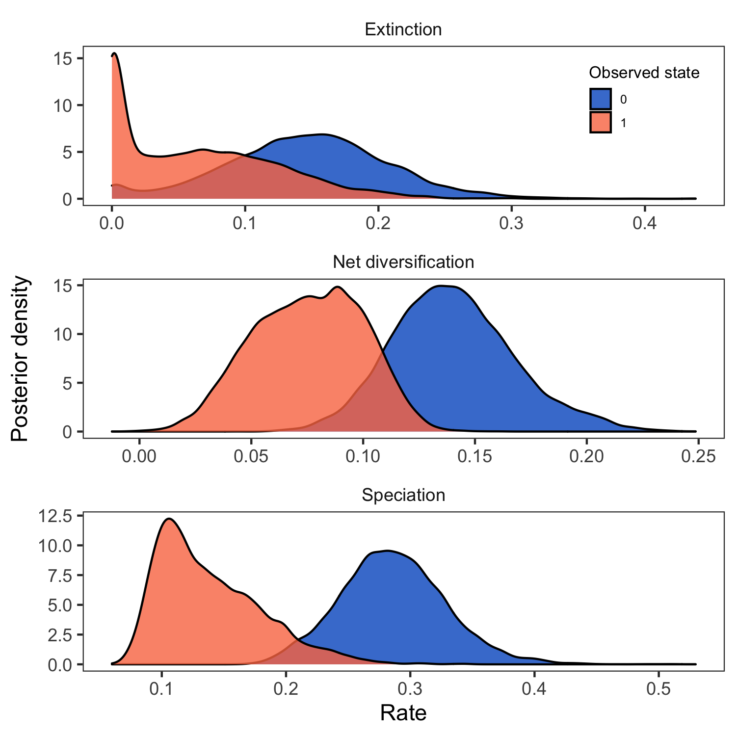
A visualization of the stochastic character map estimated under the BiSSE model. We used the script `plot_simmap_BiSSE.R`.

Summarizing Parameter Estimates

Our MCMC analysis generated a tab-delimited file called primates_BiSSE_activity_period.log that contains the samples of all the numerical parameters in our model. Again, we will use the RevGadgets (Tribble et al. 2022) R package, which allow you to generate plots and visually explore the posterior distributions of sampled parameters.

Open R.

Run this code:

library(RevGadgets)
library(ggplot2)

# read in and process the log file
bisse_file <- paste0("output/primates_BiSSE_activity_period.log")
pdata <- processSSE(bisse_file)

# plot the rates
plot <- plotMuSSE(pdata) +
        theme(legend.position = c(0.875,0.915),
              legend.key.size = unit(0.4, 'cm'), #change legend key size
              legend.title = element_text(size=8), #change legend title font size
              legend.text = element_text(size=6))

ggsave(paste0("BiSSE_div_rates_activity_period.png"),plot, width=5, height=5)

Visualizing posterior samples of the speciation rates associated with daily activity time with the `RevGadgets` (Tribble et al. 2022) R package. We used the script `plot_div_rates_BiSSE.R`.

Evaluate Social System under the BiSSE Model

Now that you have completed the BiSSE analysis for the timing of activity for all primates, perform the same analysis using a different character. Your data directory should contain the file primates_solitariness.nex, which has the coded states for each species habitat type. This is also a binary character, where the states are 0 = forest and 1 = savanna.

Complete the BiSSE analysis for habitat type using the same commands given above. Remember it is useful to clear the RevBayes console before starting another analysis. Do this using the clear() function.

While you are setting up your new analysis, substitute the character data file name so that you read in data/primates_solitariness.nex instead of primates_activity_period.nex.

It is important that you remember to also change the output file names.

View the parameter log file in Tracer after your MCMC is complete.

What is the rate of speciation associated with group living (speciation[1])? What about for solitary lineages (speciation[2])?

Compare the rate estimates
Compare the rates estimated when the activity time is the focal character versus when solitariness is the dependent character. You can do this by opening both files in the same tracer window. If you managed to give all the parameters the same name, it is possible to compare the estimates in the Tracer window by highlighting both files.

Explore the estimates of the various parameters. Are any different? Are any the same?

Why do you think you might be seeing this pattern?

Evaluate Mating System under the MuSSE Model

In RevBayes it is trivial to change the BiSSE analysis you did in the exercises above to a multi-state model that is not limited to just binary characters. That is because the model is effectively the same, just with the variable NUM_STATES changed. For this final exercise, we will use the MuSSE model (FitzJohn 2012) to estimate the rates of speciation and extinction associated with the mating system state for each primate lineage.

Your data directory should contain a file called primates_mating_system.nex. This is a four-state character where the states are: 0 = monogamy, 1 = polygyny, 2 = polygynandry, and 3 = polyandry.

Modify the analysis you completed for the binary state characters in the BiSSE Exercise to accommodate a 4-state character. This means that you must not only change the input data file (primates_mating_system.nex), but you also need to specify NUM_STATES = 4. The rate_matrix must also be modified to accommodate 4 states.

It is important that you remember to also change the output file names.

View the parameter log file in Tracer after your MCMC is complete.

What is the diversification rate associated with each state (diversification)?

Click below to begin the next exercise!

Testing for state-dependent diversification with unobserved rate variation (HiSSE)

FitzJohn R.G., Maddison W.P., Otto S.P. 2009. Estimating trait-dependent speciation and extinction rates from incompletely resolved phylogenies. Systematic Biology. 58:595–611. 10.1093/sysbio/syp067
FitzJohn R.G. 2012. Diversitree: Comparative Phylogenetic Analyses of Diversification in R. Methods in Ecology and Evolution. 3:1084–1092. 10.1111/j.2041-210X.2012.00234.x
Höhna S., Landis M.J., Heath T.A., Boussau B., Lartillot N., Moore B.R., Huelsenbeck J.P., Ronquist F. 2016. RevBayes: Bayesian Phylogenetic Inference Using Graphical Models and an Interactive Model-Specification Language. Systematic Biology. 65:726–736. 10.1093/sysbio/syw021
Kuhn T.S., Mooers A.Ø., Thomas G.H. 2011. A Simple Polytomy Resolver for Dated Phylogenies. Methods in Ecology and Evolution. 2:427–436. 10.1111/j.2041-210X.2011.00103.x
Maddison W.P., Midford P.E., Otto S.P. 2007. Estimating a binary character’s effect on speciation and extinction. Systematic Biology. 56:701. 10.1080/10635150701607033
Magnuson-Ford K., Otto S.P. 2012. Linking the Investigations of Character Evolution and Species Diversification. The American Naturalist. 180:225–245. 10.1086/666649
Tribble C.M., Freyman W.A., Landis M.J., Lim J.Y., Barido-Sottani J., Kopperud B.T., Höhna S., May M.R. 2022. RevGadgets: An R package for visualizing Bayesian phylogenetic analyses from RevBayes. Methods in Ecology and Evolution. 13:314–323. https://doi.org/10.1111/2041-210X.13750
Vos R.A., Mooers A.Ø. 2006. A New Dated Supertree of the Primates. .
Yu G., Smith D.K., Zhu H., Guan Y., Lam T.T.-Y. 2017. ggtree: an R package for visualization and annotation of phylogenetic trees with their covariates and other associated data. Methods in Ecology and Evolution. 8:28–36.