Introduction
BiSSE and MuSSE are powerful approaches for testing the association of a character with diversification rate heterogeneity. However, BiSSE has been shown to be prone to falsely identifying a positive association when diversification rate shifts are correlated with a character not included in the model (Maddison and FitzJohn 2015; Rabosky and Goldberg 2015).
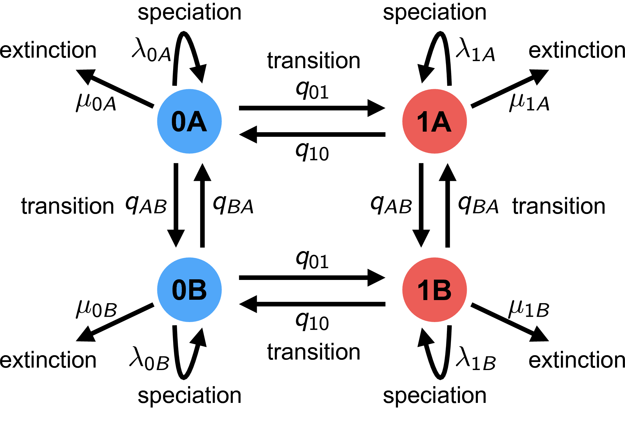
The HiSSE (Hidden State-Dependent Speciation and Extinction) model reduces the possibility of falsely associating a character with diversification rate heterogeneity (Beaulieu and O’Meara 2016). It does this by incorporating a second, unobserved character. The changes in the unobserved character’s state represent background diversification rate changes that are not correlated with the observed character. See for a schematic overview of the HiSSE model, and Table 2 for an explanation of the HiSSE model parameters.
We will keep this tutorial brief and assume that you have worked through the State-dependent diversification with BiSSE and MuSSE.
Estimating State-Dependent Speciation and Extinction under the HiSSE Model
First, we create some global variables to set-up our analysis. Using this variable we can easily change our script to use a different character with a different number of states. We will also use this variable in our second example on hidden-state speciation and extinction model.
NUM_TOTAL_SPECIES     = 367
NUM_STATES            = 2
NUM_HIDDEN            = 4
NUM_RATES             = NUM_STATES * NUM_HIDDEN
H                     = 0.587405
DATASET               = "activity_period"
Read in the Data
Begin by reading in the observed tree and the character data. We have both stored in separate nexus files.
observed_phylogeny <- readTrees("data/primates_tree.nex")[1]
data <- readCharacterData("data/primates_activity_period.nex")
It will be convenient to get some helper variables with information from the tree:
taxa <- observed_phylogeny.taxa()
tree_length <- observed_phylogeny.treeLength()
For the HiSSE model, we need to expand our characters to the new state space.
This means, that originally we had the states 0 and 1.
Now, we want to have the states 0A, 0B, 0C, 0D and 1A, 1B, 1C, 1D.
A character that was originally in state 0 will now be ambiguous for all states 0A, 0B, 0C and 0D.
Instead of coding this up manually, RevBayes provides a simple function for you.
data_exp <- data.expandCharacters( NUM_HIDDEN )
Finally, we initialize a variable for our vector of moves and monitors.
moves    = VectorMoves()
monitors = VectorMonitors()
Specify the Model
Priors on the Rates
We start by specifying prior distributions on the diversification rates. Here, we will assume an identical prior distribution on each of the speciation and extinction rates. Furthermore, we will use a log-uniform distribution as the prior distribution on each speciation and extinction rate (i.e., a uniform distribution on the log of the rates).
\(\lambda_{ij} = \lambda_{\text{observed},i} * \lambda_{\text{hidden},j}\) For example, we have $\lambda_{0A} = \lambda_{\text{observed},0} * \lambda_{\text{hidden},A}$
Let’s code this up in RevBayes.
First, we create the vector of hidden speciation rates.
Following the idea of discretizing a continuous distribution of diversification rates
(see Branch-Specific Diversification Rate Estimation), we will specify NUM_HIDDEN speciation rates
as the quantiles of a lognormal distribution.
We need the average rate of the hidden speciation rates to be fixed, because otherwise the model is not identifiable.
Therefore, we fix the median of the lognormal distribution to 1.0:
ln_speciation_hidden_mean <- ln(1.0)
Next, we draw the standard deviation of the hidden speciation rates from an exponential distribution with mean H
(so that we expect the 95% interval of the hidden speciation rate to span 1 order of magnitude).
speciation_hidden_sd ~ dnExponential( 1.0 / H )
moves.append( mvScale(speciation_hidden_sd, lambda=1, tune=true, weight=2.0) )
With the mean and the standard deviation we can specify the distribution on the hidden speciation rates. We create a deterministic variable for the hidden speciation rate categories using a discretized lognormal distribution (the N-quantiles of it).
speciation_hidden_unormalized := fnDiscretizeDistribution( dnLognormal(ln_speciation_hidden_mean, speciation_hidden_sd), NUM_HIDDEN )
However, we normalize the hidden speciation rates by dividing the rates with the main (so the mean of the normalized rates equals to 1.0):
speciation_hidden := speciation_hidden_unormalized / mean(speciation_hidden_unormalized)
Next, we repeat this same procedure for the hidden extinction rates.
ln_extinction_hidden_mean <- ln(1.0)

extinction_hidden_sd ~ dnExponential( 1.0 / H )
moves.append( mvScale(extinction_hidden_sd, lambda=1, tune=true, weight=2.0) )

extinction_hidden_unormalized := fnDiscretizeDistribution( dnLognormal(ln_extinction_hidden_mean, extinction_hidden_sd), NUM_HIDDEN )
extinction_hidden := extinction_hidden_unormalized / mean(extinction_hidden_unormalized)
For the observed speciation and extinction rates, we will apply a different approach. We will draw the speciation and extinction rates for the observed characters from identical distribution, so that a priori we expect with probability 0.5 that $\lambda_{\text{observed},0} > \lambda_{\text{observed},1}$, and with probability 0.5 we expect $\lambda_{\text{observed},1} > \lambda_{\text{observed},0}$. For the lack of prior knowledge, we specify a log-uniform prior distribution on the speciation and extinction rates for the observed characters. Note that we also initialize the starting states to make the analysis run more efficiently.
for (i in 1:NUM_STATES) {

    ### Create a loguniform distributed variable for the speciation rate
    speciation_observed[i] ~ dnLoguniform( 1E-6, 1E2)
    speciation_observed[i].setValue( (NUM_TOTAL_SPECIES-2) / tree_length )
    moves.append( mvScale(speciation_observed[i],lambda=1.0,tune=true,weight=3.0) )

    ### Create a loguniform distributed variable for the speciation rate
    extinction_observed[i] ~ dnLoguniform( 1E-6, 1E2)
    extinction_observed[i].setValue( speciation_observed[i] / 10.0 )
    moves.append( mvScale(extinction_observed[i],lambda=1.0,tune=true,weight=3.0) )

}
We have now specified the diversification rate variables for the observed and hidden states. That means, we can now put these two put together.
for (j in 1:NUM_HIDDEN) {
    for (i in 1:NUM_STATES) {
        index = i+(j*NUM_STATES)-NUM_STATES
        speciation[index] := speciation_observed[i] * speciation_hidden[j]
        extinction[index] := extinction_observed[i] * extinction_hidden[j]
    }
}
Now we can specify our character-specific speciation and extinction rate
parameters. Because we will use the same prior for each rate, it’s easy
to specify them all in a for-loop. We will use a log-uniform distribution as a prior
on the speciation and extinction rates. The loop also allows us to apply moves to each
of the rates we are estimating and create a vector of deterministic nodes
representing the rate of diversification ($\lambda - \mu$) associated with each
character state.
The stochastic nodes representing the vector of speciation rates and vector of
extinction rates have been instantiated. The software assumes that the rate in position [1] of each
vector corresponds to the rate associated with diurnal 0 lineages and the rate
at position [2] of each vector is the rate associated with nocturnal 1 lineages.
Next we specify the transition rates between the states 0 and 1:
$q_{01}$ and $q_{10}$. As a prior, we choose that each transition rate
is drawn from an exponential distribution with a mean of 10 character
state transitions over the entire tree. This is reasonable because we
use this kind of model for traits that transition not-infrequently, and
it leaves a fair bit of uncertainty.
Note that we will actually use a for-loop to instantiate the transition rates
so that our script will also work for non-binary characters.
rate_pr := observed_phylogeny.treeLength() / 10
for ( i in 1:(NUM_STATES*(NUM_STATES-1)) ) {
    transition_rates[i] ~ dnExp(rate_pr)
    moves.append( mvScale(transition_rates[i],lambda=0.50,tune=true,weight=3.0) )
}
Similarly to the rate of change between the observed character, we also add a rate of change between the unobserved character, the hidden rate. Thus, we will also assume the same exponential prior distribution.
hidden_rate ~ dnExponential(rate_pr)
moves.append( mvScale(hidden_rate,lambda=0.5,tune=true,weight=5) )
Furthermore, since there is no additional information, we assume that the rate of change between all hidden rates is identical.
for (i in 1:(NUM_HIDDEN * (NUM_HIDDEN - 1))) {
    R[i] := hidden_rate
}
Finally, we can build our rate matrix.
We do this using the specific fnHiddenStateRateMatrix function.
rate_matrix := fnHiddenStateRateMatrix(transition_rates, R, rescaled=false)
Note that we do not “rescale” the rate matrix. Rate matrices for molecular evolution are rescaled to have an average rate of 1.0, but for this model we want estimates of the transition rates with the same time scale as the diversification rates.
Prior on the Root State
Create a variable for the root state frequencies. We are using a flat Dirichlet distribution as the prior on each state. There has been some discussion about this in (FitzJohn et al. 2009). You could also fix the prior probabilities for the root states to be equal (generally not recommended), or use empirical state frequencies.
rate_category_prior ~ dnDirichlet( rep(1,NUM_RATES) )
Note that we use the rep() function which generates a vector of length NUM_STATES
with each position in the vector set to 1. Using this function and the NUM_STATES
variable allows us to easily use this Rev script as a template for a different analysis
using a character with more than two states.
We will use a special move for objects that are drawn from a Dirichlet distribution:
moves.append( mvBetaSimplex(rate_category_prior,tune=true,weight=2) )
moves.append( mvDirichletSimplex(rate_category_prior,tune=true,weight=2) )
The Probability of Sampling an Extant Species
All birth-death processes are conditioned on the probability a taxon is sampled in the present. We can get an approximation for this parameter by calculating the proportion of sampled species in our analysis.
We know that we have sampled 233 out of 367 living described primate species. To account for this we can set the sampling probability as a constant node with a value of 233/367.
rho <- observed_phylogeny.ntips()/367
Root Age
The birth-death process also depends on time to the most-recent-common ancestor–i.e., the root. In this exercise we use a fixed tree and thus we know the age of the tree.
root <- observed_phylogeny.rootAge()
The Time Tree
Now we have all of the parameters we need to specify the full character
state-dependent birth-death model. We initialize the stochastic node
representing the time tree and we create this node using the dnCDBDP() function.
timetree ~ dnCDBDP( rootAge           = root,
                    speciationRates   = speciation,
                    extinctionRates   = extinction,
                    Q                 = rate_matrix,
                    delta             = 1.0,
                    pi                = rate_category_prior,
                    rho               = rho,
                    condition         = "survival" )
Now, we will fix the HiSSE time-tree to the observed values from our data files. We use
the standard .clamp() method to give the observed tree and branch times:
timetree.clamp( observed_phylogeny )
timetree.clampCharData( data_exp )
And then we use the .clampCharData() to set the observed states at the tips of the tree:
timetree.clampCharData( data )
Finally, we create a workspace object of our whole model. The model()
function traverses all of the connections and finds all of the nodes we
specified.
mymodel = model(timetree)
Running an MCMC analysis
Specifying Monitors
For our MCMC analysis, we set up a vector of monitors to record the states of our Markov chain. The first monitor will model all numerical variables; we are particularly interested in the rates of speciation, extinction, and transition.
monitors.append( mnModel(filename="output/primates_HiSSE_activity_period.log", printgen=1) )
Optionally, we can sample ancestral states during the MCMC analysis. We need to add an additional monitor to record the state of each internal node in the tree. The file produced by this monitor can be summarized so that we can visualize the estimates of ancestral states.
monitors.append( mnJointConditionalAncestralState(tree=timetree,
                     cdbdp=timetree,
                     type="Standard",
                     printgen=1,
                     withTips=true,
                     withStartStates=false,
                     filename="output/primates_HiSSE_activity_period_anc_states.log") )
Similarly, you may want to add a stochastic character map.
monitors.append( mnStochasticCharacterMap(cdbdp=timetree,
                       filename="output/primates_HiSSE_activity_period_stoch_map.log",
                       printgen=1) )
Then, we add a screen monitor showing some updates during the MCMC run.
monitors.append( mnScreen(printgen=10, speciation, extinction) )
Initializing and Running the MCMC Simulation
With a fully specified model, a set of monitors, and a set of moves, we
can now set up the MCMC algorithm that will sample parameter values in
proportion to their posterior probability. The mcmc() function will
create our MCMC object:
mymcmc = mcmc(mymodel, monitors, moves, nruns=2, combine="mixed")
Now, run the MCMC:
mymcmc.run(generations=5000, tuningInterval=200)
Summarize Sampled Ancestral States
If we sampled ancestral states during the MCMC analysis, we can use the RevGadgets (Tribble et al. 2022) R package
to plot the ancestral state reconstruction.
First, though, we must summarize the sampled values in RevBayes.
To do this, we first have to read in the ancestral state log file. This uses a specific function called readAncestralStateTrace().
anc_states = readAncestralStateTrace("output/primates_HiSSE_activity_period_anc_states.log")
Now, we can write an annotated tree to a file. This function will write a tree with each node labeled with the maximum a posteriori (MAP) state and the posterior probabilities for each state.
anc_tree = ancestralStateTree(tree=T,
                  ancestral_state_trace_vector=anc_states,
                  include_start_states=false,
                  file="output/primates_HiSSE_anc_states_results.tree",
                  burnin=0,
                  summary_statistic="MAP",
                  site=1)
Similarly, we compute the maximum a posteriori (MAP) stochastic character map.
anc_state_trace = readAncestralStateTrace("output/primates_HiSSE_activity_period_stoch_map.log")
characterMapTree(observed_phylogeny,
                 anc_state_trace,
                 character_file="output/primates_HiSSE_activity_period_stoch_map_character.tree",
                 posterior_file="output/primates_HiSSE_activity_period_stoch_map_posterior.tree",
                 burnin=0.1,
                 reconstruction="marginal")
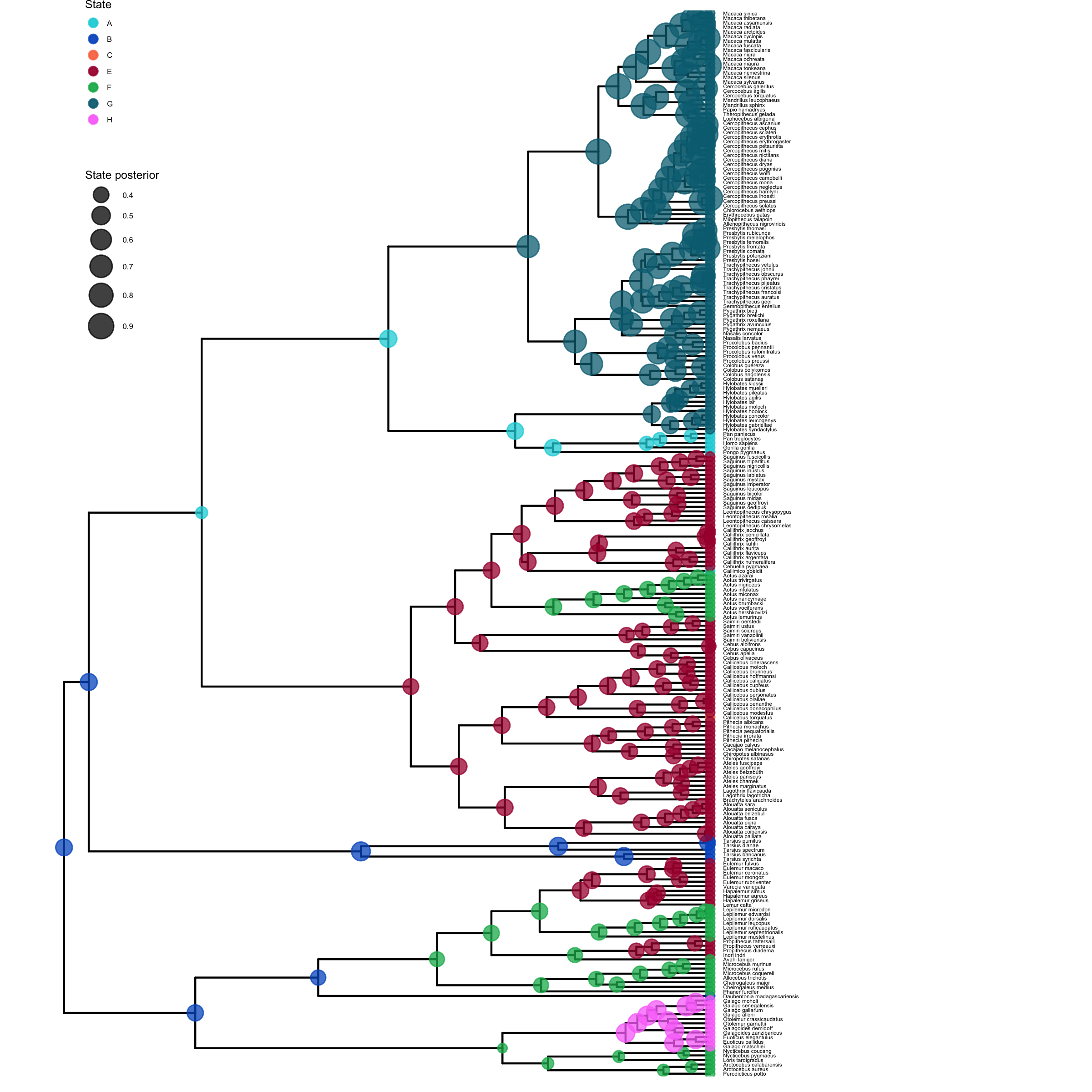
Visualize Estimated Ancestral States
To visualize the posterior probabilities of ancestral states, we will use the RevGadgets (Tribble et al. 2022) R package.
Open R.
RevGadgets requires the ggtree package (Yu et al. 2017).
First, install the ggtree and RevGadgets packages:
install.packages("devtools")
library(devtools)
install_github("GuangchuangYu/ggtree")
install_github("revbayes/RevGadgets")
Run this code (or use the script plot_anc_states_HiSSE.R):
library(ggplot2)
library(RevGadgets)

# read in and process the ancestral states
HiSSE_file <- paste0("output/primates_HiSSE_activity_period_anc_states_results.tree")
p_anc <- processAncStates(HiSSE_file)

# plot the ancestral states
plot <- plotAncStatesMAP(p_anc,
        tree_layout = "rect",
        tip_labels_size = 1) +
        # modify legend location using ggplot2
        theme(legend.position = c(0.1,0.85),
              legend.key.size = unit(0.3, 'cm'), #change legend key size
              legend.title = element_text(size=6), #change legend title font size
              legend.text = element_text(size=4))

ggsave(paste0("HiSSE_anc_states_activity_period.png"),plot, width=8, height=8)
plot_anc_states_HiSSE.R.Next, we also want to plot the stochastic character map.
Use the script plot_simmap_HiSSE.R.
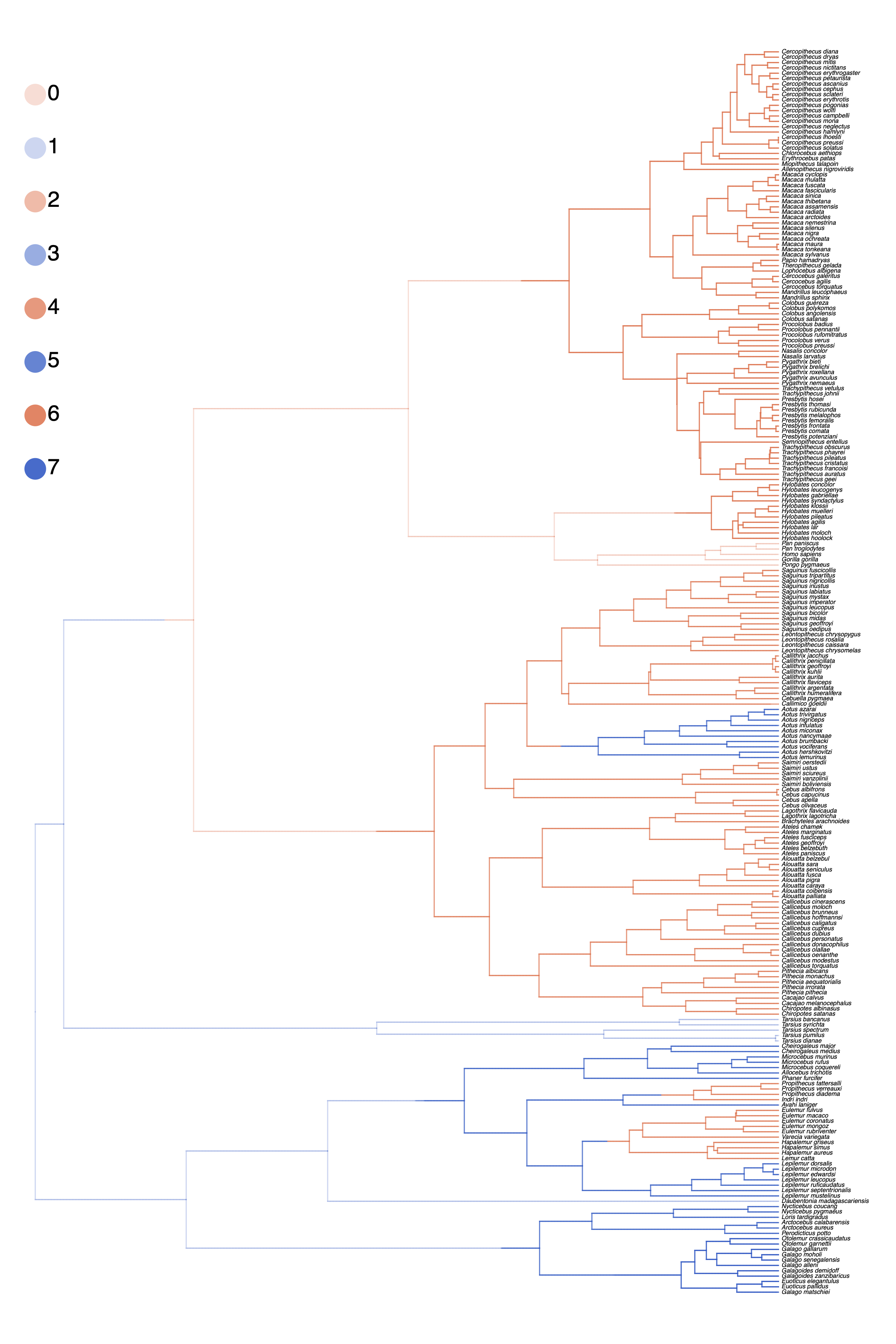
plot_simmap_HiSSE.R.Summarizing Parameter Estimates
Our MCMC analysis generated a tab-delimited file called primates_HiSSE_activity_period.log that contains
the samples of all the numerical parameters in our model.
Again, we will use the RevGadgets (Tribble et al. 2022) R package, which allow you to generate plots and
visually explore the posterior distributions of sampled parameters.
Open R.
Run this code:
library(RevGadgets)
library(ggplot2)

# read in and process the log file
HiSSE_file <- paste0("output/primates_HiSSE_activity_period.log")
pdata <- processSSE(HiSSE_file)

# plot the rates
plot <- plotMuSSE(pdata) +
        theme(legend.position = c(0.875,0.915),
              legend.key.size = unit(0.4, 'cm'), #change legend key size
              legend.title = element_text(size=8), #change legend title font size
              legend.text = element_text(size=6))

ggsave(paste0("HiSSE_div_rates_activity_period.png"),plot, width=5, height=5)
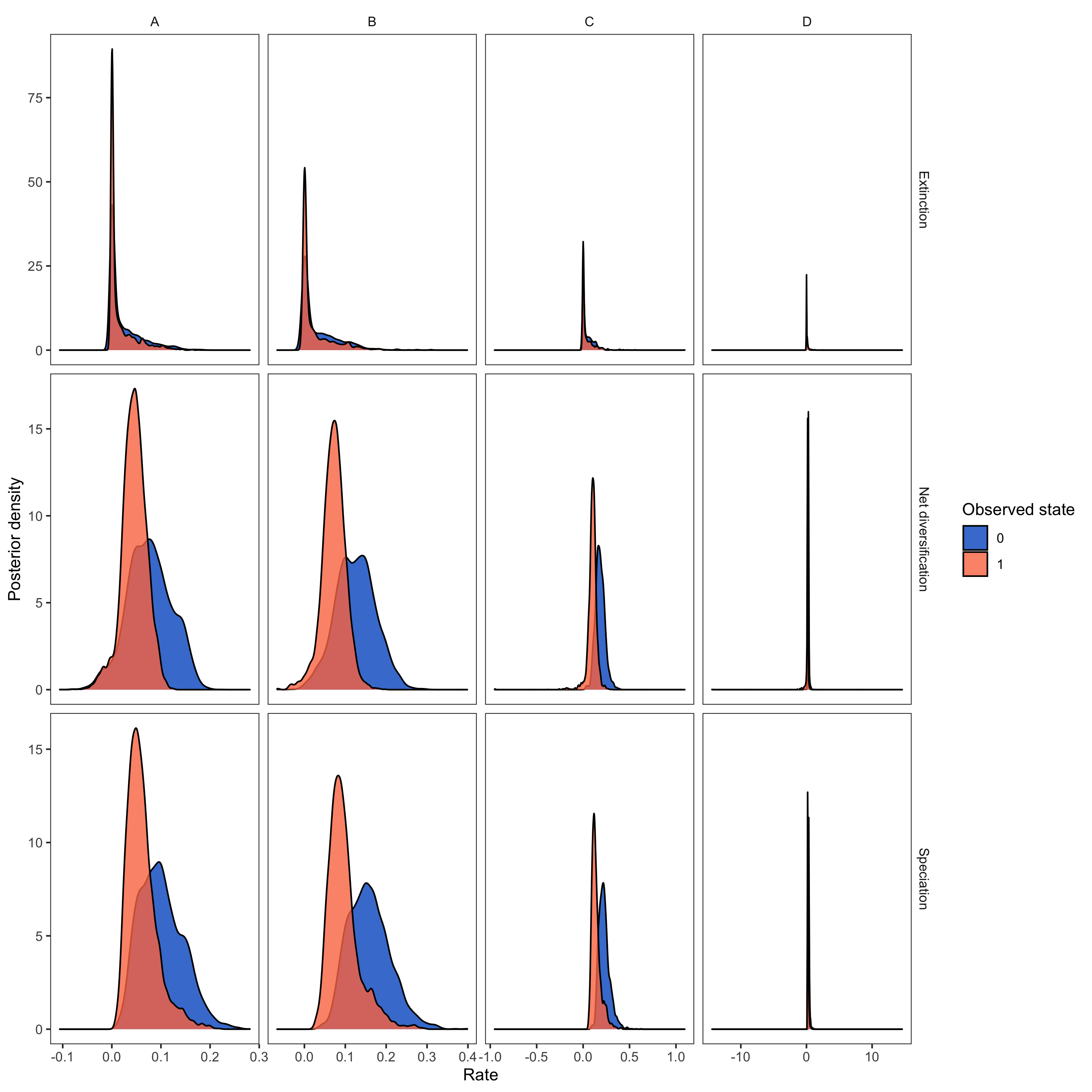
RevGadgets (Tribble et al. 2022) R package. We used the script plot_div_rates_HiSSE.R.- Beaulieu J.M., O’Meara B.C. 2016. Detecting hidden diversification shifts in models of trait-dependent speciation and extinction. Systematic Biology. 65:583–601. 10.1093/sysbio/syw022
- FitzJohn R.G., Maddison W.P., Otto S.P. 2009. Estimating trait-dependent speciation and extinction rates from incompletely resolved phylogenies. Systematic Biology. 58:595–611. 10.1093/sysbio/syp067
- Maddison W.P., FitzJohn R.G. 2015. The Unsolved Challenge to Phylogenetic Correlation Tests for Categorical Characters. Systematic Biology. 64:127–136. 10.1093/sysbio/syu070
- Rabosky D.L., Goldberg E.E. 2015. Model inadequacy and mistaken inferences of trait-dependent speciation. Systematic Biology. 64:340–355. 10.1093/sysbio/syu131
- Tribble C.M., Freyman W.A., Landis M.J., Lim J.Y., Barido-Sottani J., Kopperud B.T., Höhna S., May M.R. 2022. RevGadgets: An R package for visualizing Bayesian phylogenetic analyses from RevBayes. Methods in Ecology and Evolution. 13:314–323. https://doi.org/10.1111/2041-210X.13750
- Yu G., Smith D.K., Zhu H., Guan Y., Lam T.T.-Y. 2017. ggtree: an R package for visualization and annotation of phylogenetic trees with their covariates and other associated data. Methods in Ecology and Evolution. 8:28–36.