Introduction

In the previous examples we have modeled all character state transitions as anagenetic changes. Anagenetic changes occur along the branches of a phylogeny, within a lineage. Cladogenetic changes, on the other hand, occur at speciation events. They represent changes in a character state that may be associated with speciation events due to increased reproductive isolation, for example colonizing a new geographic area or a shift in chromosome number. Note that it can be quite tricky to determine if a character state shift is a cause or a consequence of speciation, but we can at least test if state changes tend to occur in the same time window as speciation events.

A major challenge for all phylogenetic models of cladogenetic character change is accounting for unobserved speciation events due to lineages going extinct and not leaving any extant descendants (Bokma 2002), or due to incomplete sampling of lineages in the present. Teasing apart the phylogenetic signal for cladogenetic and anagenetic processes given unobserved speciation events is a major difficulty. Commonly used biographic models like the dispersal-extinction-cladogenesis (DEC; Ree and Smith (2008)) simply ignore unobserved speciation events and so result in biased estimates of cladogenetic versus anagenetic change.

This bias can be avoided by using the Cladogenetic State change Speciation and Extinction (ClaSSE) model (Goldberg and Igić 2012), which accounts for unobserved speciation events by jointly modeling both character evolution and the phylogenetic birth-death process. ClaSSE models extend other SSE models by incorporating both cladogenetic and anagenetic character evolution. This approach has been used to model biogeographic range evolution (Goldberg et al. 2011) and chromosome number evolution (missing reference).

Here we will use RevBayes to examine biogeographic range evolution in the primates. We will model biogeographic range evolution similar to a DEC model, however we will use ClaSSE to account for speciation events unobserved due to extinction or incomplete sampling.

Setting up the analysis

Reading in the data

Begin by reading in the observed tree.

observed_phylogeny <- readTrees("data/primates_biogeo.tre")[1]

Get the taxa in the tree. We’ll need this later on.

taxa = observed_phylogeny.taxa()

Now let’s read in the biogeographic range data. The areas are represented as the following character states:

• 0 = 00 = the null state with no range
• 1 = 01 = New World only
• 2 = 10 = Old World only
• 3 = 11 = both New and Old World

For consistency, we have chosen to use the same representation of biogeographic ranges used in the \RevBayes biogeography/DEC tutorial. Each range is represented as both a natural number (0, 1, 2, 3) and a corresponding bitset (00, 01, 10, 11). The null state (state 0) is used in DEC models to represent a lineage that has no biogeographic range and is therefore extinct. Our model will include this null state as well, however, we will explicitly model extinction as part of the birth-death process so our character will never enter state 0.

data_biogeo = readCharacterDataDelimited("data/primates_biogeo.tsv", stateLabels="0123", type="NaturalNumbers", delimiter="\t", headers=TRUE)

Also we need to create the move and monitor vectors.

moves = VectorMoves()
monitors = VectorMonitors()

Set up the extinction rates

We are going to draw both anagenetic transition rates and diversification rates from a lognormal distribution. The mean of the prior distribution will be $\ln(\frac{\text{#Taxa}}{2}) / \text{tree-age}$ which is the expected net diversification rate, and the SD will be 1.0 so the 95\% prior interval ranges well over 2 orders of magnitude.

num_species <- 424 # approximate total number of primate species
rate_mean <- ln( ln(num_species/2.0) / observed_phylogeny.rootAge() )
rate_sd <- 1.0

The extinction rates will be stored in a vector where each element represents the extinction rate for the corresponding character state. We have chosen to allow a lineage to go extinct in both the New and Old World at the same time (like a global extinction event). As an alternative, you could restrict the model so that a lineage can only go extinct if it’s range is limited to one area.

extinction_rates[1] <- 0.0 # the null state (state 0)
extinction_rates[2] ~ dnLognormal(rate_mean, rate_sd) # extinction when the lineage is in New World (state 1)
extinction_rates[3] ~ dnLognormal(rate_mean, rate_sd) # extinction when the lineage is in Old World (state 2)
extinction_rates[4] ~ dnLognormal(rate_mean, rate_sd) # extinction when in both (state 3)

Note \Rev vectors are indexed starting with 1, yet our character states start at 0. So \texttt{extinction_rate[1]} will represent the extinction rate for character state 0.

Add MCMC moves for each extinction rate.

moves.append( mvSlide( extinction_rates[2], weight=4 ) )
moves.append( mvSlide( extinction_rates[3], weight=4 ) )
moves.append( mvSlide( extinction_rates[4], weight=4 ) )

Let’s also create a deterministic variable to monitor the overall extinction rate.

total_extinction := sum(extinction_rates)

Set up the anagenetic transition rate matrix

First, let’s create the rates of anagenetic dispersal:

anagenetic_dispersal_13 ~ dnLognormal(rate_mean, rate_sd) # disperse from New to Old World 01 -> 11
anagenetic_dispersal_23 ~ dnLognormal(rate_mean, rate_sd) # disperse from Old to New World 10 -> 11

Now add MCMC moves for each anagenetic dispersal rate.

moves.append( mvSlide( anagenetic_dispersal_13, weight=4 ) )
moves.append( mvSlide( anagenetic_dispersal_23, weight=4 ) )

The anagenetic transitions will be stored in a 4 by 4 instantaneous rate matrix. We will construct this by first creating a vector of vectors. Let’s begin by initalizing all rates to 0.0:

for (i in 1:4) {
    for (j in 1:4) {
        r[i][j] <- 0.0
    }
}

Now we can populate non-zero rates into the anagenetic transition rate matrix:

r[2][4] := anagenetic_dispersal_13
r[3][4] := anagenetic_dispersal_23
r[4][2] := extinction_rates[3]
r[4][3] := extinction_rates[2]

Note that we have modeled the rate of 11 $\rightarrow$ 01 (3 $\rightarrow$ 1) as being the rate of going extinct in area 2, and the rate of 11 $\rightarrow$ 10 (3 $\rightarrow$ 2) as being the rate of going extinct in area 1.

Now we pass our vector of vectors into the \cl{fnFreeK} function to create the instaneous rate matrix.

ana_rate_matrix := fnFreeK(r, rescaled=false)

Set up the cladogenetic speciation rate matrix

Here we need to define each cladogenetic event type in the form [ancestor\_state, daughter1\_state, daughter2\_state] and assign each cladogenetic event type a corresponding speciation rate.

The first type of cladogenetic event we’ll specify is widespread sympatry. Widespread sympatric cladogenesis is where the biogeographic range does not change; that is the daughter lineages inherit the same range as the ancestor. In this example we are not going to allow the speciation events like 11 $\rightarrow$ 11, 11, as it seems biologically implausible. However if you wanted you could add this to your model.

Define the speciation rate for widespread sympatric cladogenesis events:

speciation_wide_sympatry ~ dnLognormal(rate_mean, rate_sd)
moves.append( mvSlide( speciation_wide_sympatry, weight=4 ) )

Define the widespread sympatric cladogenetic events:

clado_events[1] = [1, 1, 1] # 01 -> 01, 01
clado_events[2] = [2, 2, 2] # 10 -> 10, 10

and assign each the same speciation rate:

speciation_rates[1] := speciation_wide_sympatry/2
speciation_rates[2] := speciation_wide_sympatry/2

Subset sympatry is where one daughter lineage inherits the full ancestral range but the other lineage inherits only a single region.

speciation_sub_sympatry ~ dnLognormal(rate_mean, rate_sd)
moves.append( mvSlide( speciation_sub_sympatry, weight=4 ) )

Define the subset sympatry events and assign each a speciation rate:

clado_events[3] = [3, 3, 1] # 11 -> 11, 01
clado_events[4] = [3, 1, 3] # 11 -> 01, 11
clado_events[5] = [3, 3, 2] # 11 -> 11, 10
clado_events[6] = [3, 2, 3] # 11 -> 10, 11
speciation_rates[3] := speciation_sub_sympatry/4
speciation_rates[4] := speciation_sub_sympatry/4
speciation_rates[5] := speciation_sub_sympatry/4
speciation_rates[6] := speciation_sub_sympatry/4

Allopatric cladogenesis is when the two daughter lineages split the ancestral range:

speciation_allopatry ~ dnLognormal(rate_mean, rate_sd)
moves.append( mvSlide( speciation_allopatry, weight=4 ) )

Define the allopatric events:

clado_events[7] = [3, 1, 2] # 11 -> 01, 10
clado_events[8] = [3, 2, 1] # 11 -> 10, 01
speciation_rates[7] := speciation_allopatry/2
speciation_rates[8] := speciation_allopatry/2

Now let’s create a deterministic variable to monitor the overall speciation rate:

total_speciation := sum(speciation_rates)

Finally, we construct the cladogenetic speciation rate matrix from the cladogenetic event types and the speciation rates.

clado_matrix := fnCladogeneticSpeciationRateMatrix(clado_events, speciation_rates, 4)

Let’s view the cladogenetic matrix to see if we have set it up correctly:

clado_matrix

Set up the cladogenetic character state-dependent birth-death process

For simplicity we will fix the root frequencies to be equal except for the null state which has probability of 0.

root_frequencies <- simplex([0, 1, 1, 1])

rho is the probability of sampling species at the present:

rho <- observed_phylogeny.ntips()/num_species

Now we construct a stochastic variable drawn from the cladogenetic character state-dependent birth-death process.

classe ~ dnCDCladoBDP( rootAge         = observed_phylogeny.rootAge(),
                       cladoEventMap   = clado_matrix,
                       extinctionRates = extinction_rates,
                       Q               = ana_rate_matrix,
                       delta           = 1.0,
                       pi              = root_frequencies,
                       rho             = rho,
                       condition       = "time",
                       taxa            = taxa )

Clamp the model with the observed data.

classe.clamp( observed_phylogeny )
classe.clampCharData( data_biogeo )

Finalize the model

Just like before, we must create a workspace model object.

mymodel = model(classe)

\subsection{Set up and run the MCMC}

First, set up the monitors that will output parameter values to file and screen.

monitors.append( mnModel(filename="output/primates_ClaSSE.log", printgen=1) )
monitors.append( mnJointConditionalAncestralState(tree=observed_phylogeny, cdbdp=classe, type="NaturalNumbers", printgen=1, withTips=true, withStartStates=true, filename="output/anc_states_primates_ClaSSE.log") )
monitors.append( mnScreen(printgen=1, speciation_wide_sympatry, speciation_sub_sympatry, speciation_allopatry, extinction_rates) )

Now define our workspace MCMC object.

mymcmc = mcmc(mymodel, monitors, moves)

We will perform a pre-burnin to tune the proposals and then run the MCMC. Note that for a real analysis you would want to run the MCMC for many more iterations.

mymcmc.burnin(generations=200,tuningInterval=5)
mymcmc.run(generations=1000)

Summarize ancestral states

When the analysis has completed you now summarize the ancestral states. The ancestral states are estimated both for the “beginning” and “end” state of each branch, so that the cladogenetic changes that occurred at speciation events are distinguished from the changes that occurred anagenetically along branches. Make sure the include_start_states argument is set to true.

anc_states = readAncestralStateTrace("output/anc_states_primates_ClaSSE.log")
anc_tree = ancestralStateTree(tree=observed_phylogeny, ancestral_state_trace_vector=anc_states, include_start_states=true, file="output/anc_states_primates_ClaSSE_results.tree", burnin=0, summary_statistic="MAP", site=0)

Plotting ancestral states

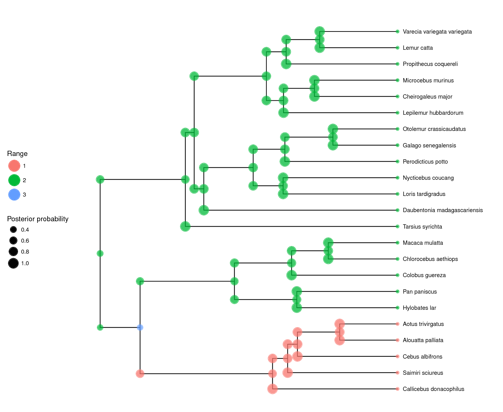
Like before, we’ll plot the ancestral states using the RevGadgets R package. Execute the script plot_anc_states_ClaSSE.R in R. The results can be seen in Figure \ref{fig:results_ClaSSE}. The maximum a posteriori (MAP) estimate for each node is shown as well as the posterior probability of the states represented by the size of the dots.

library(RevGadgets)

tree_file = "output/anc_states_primates_ClaSSE_results.tree"

plot_ancestral_states(tree_file, summary_statistic="MAPRange",
                      tip_label_size=3,
                      tip_label_offset=1,
                      xlim_visible=c(0,100),
                      node_label_size=0,
                      shoulder_label_size=0,
                      include_start_states=TRUE,
                      show_posterior_legend=TRUE,
                      node_size_range=c(4, 7),
                      alpha=0.75)

output_file = "RevBayes_Anc_States_ClaSSE.pdf"
ggsave(output_file, width = 11, height = 9)

Exercise

• Using either R or Tracer, visualize the posterior estimates for different types of cladogenetic events. What kind of speciation events are most common?
• As we have specified the model, we did not allow cladogenetic long distance (jump) dispersal, for example 01 $\rightarrow$ 01, 10. Modify this script to include cladogenetic long distance dispersal and calculate Bayes factors to see which model fits the data better. How does this affect the ancestral state estimate? }

1. Bokma F. 2002. Detection of punctuated equilibrium from molecular phylogenies. Journal of Evolutionary Biology. 15:1048–1056. 10.1046/j.1420-9101.2002.00458.x
2. Goldberg E.E., Lancaster L.T., Ree R.H. 2011. Phylogenetic Inference of Reciprocal Effects between Geographic Range Evolution and Diversification. Systematic Biology. 60:451–465. 10.1093/sysbio/syr046
3. Goldberg E.E., Igić B. 2012. Tempo and Mode in Plant Breeding System Evolution. Evolution. 66:3701–3709. 10.1111/j.1558-5646.2012.01730.x
4. Ree R.H., Smith S.A. 2008. Maximum Likelihood Inference of Geographic Range Evolution by Dispersal, Local Extinction, and Cladogenesis. Systematic Biology. 57:4–14. 10.1080/10635150701883881